Quantcast
Channel: Daily Dose of Excel
Viewing all 366 articles
Browse latest View live

Excel isn’t fully cooked.

$
0
0

It’s still raw in the middle, a bit.

  • PivotTables are great, but why can’t I filter one based on an external range?
  • Shape Styles would be cool, if I could add my own styles.
  • Slicers are great, but why isn’t there an easy way to instantly get an overview of what Slicers are connected to what PivotTables, and at the same time use the same interface to effortlessly manage this and set up exclusions?
  • Charts are great, but why do I have to manually cut and paste them many times in order to make up the equivalent of a Small Multiple chart?

Fortunately, in most cases Excel is pretty programmable. If it doesn’t do something out of the box – or if using the built-in functionality is tedious – then given the requisite skills or the right Google search then you can almost always work around such bottlenecks fairly efficiently.

Unfortunately, Excel isn’t fully programmable no matter what skills you have. The Partial Text Search box that you can use to manually filter PivotFields on partial text pretty much instantly is awesome. But you can’t address it via VBA…it’s for humans only. Which means you’ve got to iterate through potentially large PivotItems collections s-l-o-w-l-y in maybe minutes in order to do something that users can do in seconds. (I won’t mention VBA support for PowerPivot as another example, because PowerPivot is still fairly new. Rough rule of thumb: Don’t complain about something until it’s been sitting around at least 5 years in an unfinished state. At least, that’s what I tell my wife).

I’ve got some great code to handle the Filtering Pivots and the Slicers things. And I can code up a cut and paste thing for Charts pretty easily. But that Partial Text Search box I can’t help you with. Maybe this will help get it on someone’s radar, but obviously including such ‘niceties’ in the in-box functionality isn’t trivial. Otherwise the dialog box for MSQuery (which I still use) would let me expand it. And the Name Manager would let me do the things that the better Name Manager will do. And so on.

So presumably these things are not trivial to enhance, or they would be enhanced already. But here’s the thing: by comparison, my code for filtering pivots or managing Slicers is trivial to roll out to users compared to the effort required to add this functionality natively.

So question: Why don’t MS supplement their great unfinished app by building and offering to users useful workarounds in one of the most agile-ready platforms there is…VBA? Why aren’t they monitoring forums and blogs for the best and brightest productivity enhancements, and buying the IP from content creators at a song, then offering it to users as add-ins that plug the gap until they get around to finishing Excel?

Regards,
Jeff Weir.
Cosmetic Surgeon.


PivotItems Are Wrong when Calculated Field Is Present

$
0
0

I have a procedure where I loop through a pivot table and create a general journal entry to be imported. I used the same procedure to create another journal entry, but with one change. For this new journal entry, I wanted to round all of the amounts to the nearest $10. They were estimates and I don’t like to post estimates to the penny because it implies a precision that just isn’t there.

To accomplish this seemingly simple task, I created a calculated field and adjusted the procedure to pull from that field. There was just one problem: my debits didn’t equal my credits! I know, I gasped too.

It turns out that looping through the pivot table with For Each pi In pf.PivotItems was starting on the row below the first pivot item and ending on the row below the last pivot item. It was offset one row.

I was puzzled for quite a while. The old procedure worked fine. Then it dawned on me that I had added a calculated field. When I removed the calculated field, it worked as expected. So I modified the procedure to do the rounding in VBA.

Next, I wanted to see if this was a fluke. I generated some sample data, namely First Name, Last Name, and City. Then I created a pivot table with City in the Row Labels section and Count of Last in the Value section. Finally, I created a calculated field expertly named Field1.

The calculated field is set to zero. It’s not really calculating anything. I added that to the Values section.

Now to test. I wrote some code to demonstrate that the PivotItems were pointing to the wrong cells. As part of my code, I wanted to remove the calculated field. I kept getting errors trying to remove the calculated field so I recorded a macro to see how it’s supposed to be done.

ActiveSheet.PivotTables("PivotTable1").PivotFields("Sum of Field1").Orientation = xlHidden

Yep, that’s what I was trying to do. Only that doesn’t work. So I found a work around. I love finding bugs when I’m investigating other bugs.

Here’s the code:

Sub TestPivotItems()
   
    Dim pt As PivotTable
    Dim pf As PivotField
    Dim pi As PivotItem
   
    Set pt = ActiveCell.PivotTable
    Set pf = pt.PivotFields("City")
    Set pi = pf.PivotItems(1)
   
    Debug.Print pi.LabelRange.Address, pi.LabelRange.Value
    Debug.Print ActiveSheet.Cells.Find(pi.Value).Address, pi.Value
    Debug.Print String(40, "-")
   
    pt.PivotFields("Sum of Field1").DataRange.Cells(1).PivotItem.Visible = False
   
    Debug.Print pi.LabelRange.Address, pi.LabelRange.Value
    Debug.Print ActiveSheet.Cells.Find(pi.Value).Address, pi.Value
   
End Sub

And here’s the result:

Above the dashed line is what happens when calculated field is present. The PivotItem, which is in A4, shows A5 as its LabelRange. When I search for its Value, however, I get A4. When I removed the calculated field, it all works as expected.

This Database Has Been Opened Read-only when Used in External Data Table

$
0
0

If you use the From Access button on the Data Ribbon to create External Data, it uses OLEDB to link the data. In the bad ol’ days it used ODBC. Almost always when I bring data from Access to Excel, I need to open Access to fix the query or do something different. If the Excel workbook is still open, I get this unfriendly message:

This database has been opened read-only. You can only change data in linked tables. To make design changes, save a copy of the database

For some reason, the connection string created by Excel includes Mode=Share Deny Write and that causes the read-only message.

As far as I know, Excel can’t write data back to Access via the user-interface. I’d be happy to be proven wrong on that point – and very surprised. So why not just make the connection string read-only?

Fortunately, you can edit the connection string right there in the Connection Properties dialog. I changed the Mode to Mode=Read, and it fixes the problem.

If the database is open in Access at the time I create the external data table, it prompts me for data link properties. On the Advanced tab, I can change the mode. So I guess that’s easier than going through the connection properties after the fact.

Sadly, there’s no specific event for adding an external data table. If there were, I could change that setting for every new table added. I could use the Worksheet_Change event, but I don’t want that code running for every change in every worksheet. That would be crazy. So I’m stuck fixing it manually. And by manually, I mean clicking a button.

Sub MakeExternalDataReadOnly()
   
    Dim qt As QueryTable
   
    On Error Resume Next
        Set qt = ActiveCell.ListObject.QueryTable
       
        If qt Is Nothing Then Set qt = ActiveSheet.ListObjects(1).QueryTable
    On Error GoTo 0
   
    If Not qt Is Nothing Then
        qt.Connection = Replace(qt.Connection, "Mode=Share Deny Write", "Mode=Read")
    End If
   
End Sub

If the active cell is in a listobject that has external data, assume that’s the one to change. If not, assume we want to change the first one on the active sheet. If neither of those things work, don’t do anything, otherwise replace the Mode section of the connection string. Here’s the workflow:

  1. Create an external data table
  2. Open the database in Access
  3. Curse yourself for forgetting to change the connection string
  4. Run the above macro
  5. Re-open the database in Access

A date with PivotItems

$
0
0

Howdy, folks. Jeff here again. I’ve been sharpening up some code to manually filter a PivotField based on an external list in a range outside the PivotTable. It works blazingly fast. Unless there’s dates as well as non-dates in my PivotField. In which case it errors out.

Try this:
Put “Pivot” in A1
Put =TODAY() in A2
Put =VALUE(TODAY()) in A3

Now make a PivotTable out of that data.

Pivot_DDOE

Now put this code into the VBE and step through it:

Sub WhatThe()

Dim pf As PivotField
Set pf = ActiveSheet.PivotTables(1).PivotFields(1)
With pf
    .NumberFormat = "d/mm/yyyy"
    .PivotItems(1).Visible = True
    .PivotItems(2).Visible = True
    .NumberFormat = "General"
    .PivotItems(1).Visible = True
    .PivotItems(2).Visible = True
End With
End Sub

If the same thing happens to you as happens to me, you will either be speaking aloud the title of this routine, or you will be speaking aloud this:
Unable to get the PivotItems property of the PivotField class.

Go type these in the immediate pane:

? .PivotItems(1).name
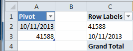
41588
? .PivotItems(1).visible
True
? .PivotItems(2).name
10/11/2013
? .PivotItems(2).visible
Error 2042

What the…?

Now try these:

? ActiveSheet.PivotTables(1).PivotFields(1).numberformat
General
ActiveSheet.PivotTables(1).PivotFields(1).numberformat = "d/mm/yyyy"
? .PivotItems(2).name
10/11/2013
? .PivotItems(2).visible
True

So it seems can’t do certain stuff to a PivotItem if that PivotItem is a date but your PivotField number format is set to General.

That’s weird.

Equally weird, try this:
Select the PivotTable, and record a macro as you change it’s number format back to General.

Sub WhatThe_Part2()  
 ActiveSheet.PivotTables("PivotTable14").PivotFields("Pivot").Name = "General"
End Sub

What the …? Change the PivotField Number Format, and you get a macro that tells you that you changed the PivotField name!

So what happens if you run that macro? Well, it changes the name of the PivotField:
PivotField_20131110

It does nothing to the number format.

Strangely enough, I found some info on this problem at one of my most revisited blogposts that I had somehow missed: Jon Peltier’s Referencing Pivot Table Ranges in VBA

Stranger still, the answer was by Jon Peltier back in 2009 in relation to a question asked by….wait for it…me. Don’t know how I missed that. Must have been sleeping.
So I’ve come across this problem before, found an answer, completely forgotten about it, and then wasted 2 days trying to work out what the problem was, purely so I could Google my own answered question.

I’m going to read through all 238 ( and counting) comments in that thread and see what else Jon has told me over the years I’ve been learning VBA.
There’s also something on this at stackoverflow

Jeff

–edit–
Jon’s method was to loop through the pivot items, and compare the pivot item caption to what he was looking for:

For Each pi In pt.PivotFields("Order Month/Year").PivotItems
  If pi.Caption = Format(TheDate, "m/dd/yyyy") Then
  ' or If DateValue(pi.Caption) = TheDate Then
    '' FOUND IT
  End If
Next

But now I know it’s probably easier just to change the format of the PivotField.

Repeating Values in Pivot Tables

$
0
0

Often I’m using a PivotTable to aggregate some data to use elsewhere. I’ll take a PivotTable that looks like this

and make it look like a grid so that I can copy and paste it somewhere else. To do that, I first go to the PivotTable Options – Display tab and change it to Classic PivotTable layout.

Then I’ll go to each PivotItem that’s a row and remove the subtotal

and check the Repeat item labels checkbox.

And I get a PivotTable that’s ready for copying and pasting.

After about 50 times of doing that, I got sick of it. Now I just run this code.

Sub PivotGrid()
       
    Dim pt As PivotTable
    Dim pf As PivotField
   
    On Error Resume Next
        Set pt = ActiveCell.PivotTable
    On Error GoTo 0
   
    If Not pt Is Nothing Then
        With pt
            .InGridDropZones = True
            .RowAxisLayout xlTabularRow
        End With
       
        For Each pf In pt.PivotFields
            If pf.Orientation = xlRowField Then
                pf.Subtotals = Array(False, False, False, False, False, False, False, False, False, False, False, False)
                pf.RepeatLabels = True
            End If
        Next pf
    End If
   
End Sub

Filtering Pivots based on external ranges.

$
0
0

Howdy, folks. Jeff here again. We might as well rename this blog Daily Dose of Pivot Tables, because here’s yet another treatment of this well-worn subject this week.

Let’s say you’ve got a PivotField with 20,000 items in it. What’s the quickest way to filter that PivotTable based on an external list that contains either 100, 10000, or 19900 of those items?
The usual approach to a task like this is to just iterate through each pivotitem in the PivotItems collection, and check if that PivotItem is in the list of search terms. If it is, you make the PivotItem visible, otherwise you hide it.

But this requires us to:

  • Read the PivotItem name
  • Read in the Search Terms
  • Check if each PivotItem is in the list of search terms. If it is, you make the PivotItem visible, otherwise you hide it.

How long does each part of this take? Where are the bottlenecks? Let’s find out.

First, how long does it take just to iterate through all 20,000 items and get the value of each PivotItem? (Note that I’ve set pt.ManualUpdate = True before running all the following snippets, so that the PivotTable doesn’t try to update after each and every change)

For Each pi In pf.PivotItems
    strName = pi.Value 'In my test data, all items are strings
Next

Not long at all. Under a second.

How long to work out what the current visiblestatus is of each PivotItem?

For Each pi In pf.PivotItems
    bStatus = pi.Visible
Next

One minute and twenty seconds? Really? Not exactly lightning fast, is it?

Okay, how long does it take to set the .Visible property of each item, without checking what it currently is? Let’s set .visible = true for each and every PivotItem (even though they are already visible) just to find out what the worst case scenario is.

For Each pi In pf.PivotItems
    pi.Visible = True
Next

Two minutes, 43 seconds. So it takes longer to set the .visible status than to read it. Handy to know.

Okay, how long will it take to first check the .Visible property of each item, and then change it?

For Each pi In pf.PivotItems
    pi.Visible = Not pi.Visible
Next

Four minutes, 26 seconds. Not surprising I guess, because it’s got to first find the current state of each item – which we already established above takes around one minute and twenty seconds – and then we need to change the state – which we already established above takes around 2 minutes 43 seconds. And those two times add up to 4 minutes.

So that’s how long it would take in principle to filter the PivotTable based on the initial approach I suggested above, excluding the time taken to actually check for duplicates between the PivotItems and the search terms.

Ahhh… I hear you say (I have good ears). What if we first check whether the .visible status of a PivotItem is already set how we want it. That way, we can save some time by only changing it if it actually needs to be changed. Good point, and nice to see you’re alert.

So here’s our efficient tweak of the ‘traditional’ method:

  • Add all Search terms to a dictionary (or collection, if you prefer)
  • Try to add each PivotItem to that same dictionary.
  • If that last step caused an error, we’ll know that this PivotItem is in our list of search terms. In this case, we can check what the current visible status is of the PivotItem. If it’s NOT visible, we’ll make it visible. If it IS visible, we do nothing
  • IF this didn’t cause an error, we’ll know that this PivotItem IS NOT in our list of filter terms. In this case, we again check what the current visible status is of the PivotItem. If it’s visible, we’ll hide it. If it’s already hidden, we do nothing

So this approach is quite efficient in that it only changes the .visible status of the PivotItem if it has to. Which is good, because this is the bottleneck. And the general approach of using a Dictionary (or collection) is very efficient, compared to other ways I’ve seen on line that use say applicaiton.match to check the PivotItem against a variant array or (far worse) against the original FilterTerms range in the worksheet.

On a pivot of 20,000 items that currently has all items visible, here’s how this ‘tweaked traditional’ method performed:

  • It took 4:21 to filter on a list of 100 terms. When I ran it again without clearing the filter, it only took 1:32. That faster time is because it didn’t have to change the .visible status of any items at all, because they were already in the ‘correct’ state after the last run. But it still had to check them all
  • It took 3:03 to filter on a list of 10,000 terms. The shorter time compared to the first test case is because it only had to set the .visible status of half the pivot items. It took 1:35 when I ran it again without clearing the filter, same as before. That’s what I would expect.
  • It took 1:35 again to filter on a list of 19900 items – the same as the 2nd pass in the other cases, which again is what I would expect given it only had to hide a few items. And of course it took about the same time again when I ran it again without clearing the filter, same as before.

(Note that my ‘tweaked traditional’ routine has some extra checks to handle errors caused by dates in PivotFields not formatted as Date Fields, something I discussed here. And it also has to do some extra checking for PivotItems such as “1.1″, because VBA’s IsDate function interprets such a string as a date. But the extra processing time of these extra loops is pretty inconsequential compared to checking and changing the .Visible status.)

Can we do better than that?

Of course we can. What if we work out how many PivotItems in the PivotField, and how many search terms in the Search list, and either make all PivotItems visible or all PivotItems (bar one) hidden before we start, so that we minimise the amount of PivotItems we have to change the .Visible status of?

  • If there’s just 100 items in our Search Terms list, hide all but one PivotItem, then unhide just the 100 matching items
  • If there’s 19900 items in our Search Terms list, make all PivotItems visible, then hide the 100 PivotItems that are not in the Search Terms list
  • Because we know in advance whether all PivotItems are visible or hidden, we don’t have to check their .visible status at all.

Genius in theory, I know. And it’s certainly trivial to clear a PivotFilter so that all items are visible in that 2nd case. But that 1st case is tricky: how do you hide all but one PivotItem via VBA without iterating through and having to do all that incredibly slow .visible = false stuff? You can do it manually very easily of course. But via VBA? You can’t do it directly except if you make the field a Page Field and set .EnableMultiplePageItems to False. And then as soon as you change it to True again, VBA helpfully clears the filter so that all items are visible again. And so you’re back to square 1.

Enter the slicer

It turn out that you can very quickly hide all but one PivotItem programatically if you make a temp copy of the Pivot, make the field of interest in the temp into a Page field with .EnableMultiplePageItems set to False, and then hook it up via a slicer to your original Pivot. This forces the original PivotField to have the same filter setting – just one item visible. But it doesn’t make that original Pivot have the same layout. So the original pivot can still be say a Row field where you can then merrily make additional items visible.

How fast is this approach? Very. Again, using a test pivot with 20,000 items in it:

  • Filter on 100 search terms: 0:05 (compared with 4:21 in the approach above)
  • Filter on 10,000 search terms: 1:26 (compared with 3:03 in the approach above)
  • Filter on 19,900 search terms: 0:03 (compared with 1:35 in the approach above)

Now that is some improvement.

Here’s the two routines below for your viewing pleasure. I turned both routines into functions, which you call by a wrapper. This lets you pre-specify what PivotField you want to filter and where your search terms are. Otherwise you’ll be prompted to select them via some input boxes.

Also check out the attached workbook that has the code inside, and that lets you generate random alphanumeric PivotFields and Search Terms in a jiffy (something I’ll cover in a future post). Just click the Create Sample Data button after changing the input parameters, and then click on the command button of choice. When you run the code from the command buttons, the times of each pass will be recorded in the workbook too, so you can compare different settings.

Filter PivotTable 20131114

Have at it people. Look forward to comments, feedback, suggestions, and Nobel Prize nominations.

Regards,
Jeff

Slower Approach

Sub Dictionary_Slower()
FilterPivot_Dictionary_Slower
End Sub


Private Function FilterPivot_Dictionary_Slower(Optional rngPivotField As Range, Optional rngFilterItems As Range) As Boolean
' Copyright ©2013 Jeff Weir
' weir.jeff@gmail.com
' You are free to use this code within your own applications, add-ins,
' documents etc but you are expressly forbidden from selling or
' otherwise distributing this source code without prior consent.
' This includes both posting free demo projects made from this
' code as well as reproducing the code in text or html format.
' ---------------------------------------------------------------------

'   Date        Initial     Details                 Version
'   20131113    JSW         Initial Programming     007 (of course)
 
'#############
'#  Remarks  #
'#############

'   This code needs to be called by a wrapper function.
'   e.g.

'    Sub FilterPivot()
'    FilterPivot_Dictionary_Slower
'    End Sub

'   If required, that wrapper function can also provide ranges
'   specifying what PivotField to filter, and where the range of
'   filter terms is. e.g.:
'       FilterPivot_Dictionary_Slower Range("A2"), Range("C2:C20000")
'   ...or
'       FilterPivot_Dictionary_Slower(ActiveCell, [tblFilterItems])


    Dim ptOriginal As PivotTable
    Dim pfOriginal As PivotField
    Dim pfFilterItems As PivotField
    Dim pi As PivotItem
    Dim ptFilterItems As PivotTable
    Dim wksTemp As Worksheet
    Dim wksPivot As Worksheet
    Dim dic As Object
    Dim varContinue As Variant
    Dim strMessage As String
    Dim varFormat As Variant
    Dim bDateFormat As Boolean
    Dim bDateWarning As Boolean
   
   
    FilterPivot_Dictionary_Slower = False   'Assume failure

    On Error GoTo ErrHandler
    Set wksPivot = ActiveSheet

    'If neccessary, prompt user for the pivotfield of interest
    If rngPivotField Is Nothing Then
        On Error Resume Next
        Set rngPivotField = ActiveCell
        Set pfOriginal = rngPivotField.PivotField    'Tests if this is in fact a PivotField
        If Err <> 0 Then
            Err.Clear
            Set rngPivotField = Nothing
            Set rngPivotField = Application.InputBox( _
                                Title:="Where is the PivotField?", _
                                Prompt:="Please select a cell in the PivotField you want to filter", _
                                Type:=8)
            On Error GoTo ErrHandler
            If rngPivotField Is Nothing Then Err.Raise 996
        End If
        On Error GoTo ErrHandler
    End If

    Set pfOriginal = rngPivotField.PivotField
    Set ptOriginal = pfOriginal.Parent


    'If neccessary, prompt user for FilterItems table related to the pivotfield of interest
    If rngFilterItems Is Nothing Then
        On Error Resume Next
        Set rngFilterItems = Application.InputBox( _
                             Title:="Where are the filter items?", _
                             Prompt:="Please select the range where your filter terms are", _
                             Type:=8)
        On Error GoTo ErrHandler
        If rngFilterItems Is Nothing Then Err.Raise 996
    End If


    Application.ScreenUpdating = False
    Application.Calculation = xlCalculationManual
   
    ' Excel stores dates differently between PivotItems and Variant Arrays.
   
    ' For instance:
    '    ? CStr(varFilterItems(i, 1))
    '    1/01/2013
    '    ? pi.Value
    '    1/1/2013
    '    ? CStr(varFilterItems(i, 1)) = pi.Value
    '    False

    'So we 'll turn our FilterItems into a PivotTable to ensure formats are treated the same.

    Set wksTemp = Sheets.Add
    rngFilterItems.Copy wksTemp.Range("A2")
    wksTemp.Range("A1").Value = "FilterItems"
    Set rngFilterItems = wksTemp.Range("A2").CurrentRegion
   
On Error GoTo 0

    ActiveWorkbook.PivotCaches.Create(SourceType:=xlDatabase, SourceData:= _
        rngFilterItems).CreatePivotTable _
        TableDestination:=[C1], TableName:="appFilterItems"
         
    Set ptFilterItems = wksTemp.PivotTables("appFilterItems")
    Set pfFilterItems = ptFilterItems.PivotFields(1)

     ' Add FILTERItems to a Dictionary
        Set dic = CreateObject("scripting.dictionary")
        For Each pi In pfFilterItems.PivotItems
            dic.Add pi.Value, 1  'The one does nothing
        Next

    ptOriginal.ManualUpdate = True  'dramatically speeds up the routine, because the pivot won't recalculate until we're done

       
    'Check if PFOriginal is formatted as a date field.
    ' Basically there is a bug in Excel whereby if you try to do some things
    ' to a PivotItem containing a date but the PivotField number format is NOT a date format
    ' then you get an error.
    ' So we'll check the PivotField date format and see what it is
    ' Note that if a PivotField is based on a range that contains multiple formats
    ' then you get an error simply by checking what the PivotField number format is.
    ' So we'll instigate an On Error Resume Next to handle this
   
    On Error Resume Next
    varFormat = pfOriginal.NumberFormat
    On Error GoTo ErrHandler
    If IsDate(Format(1, varFormat)) Then bDateFormat = True
   
       
        ' Now try and add the PivotItems.
        ' If ther's an error, we'll know that this item is also in the FilterTerms
        On Error Resume Next
        With dic
            For Each pi In pfOriginal.PivotItems
                dic.Add pi.Value, 1 'The 1 does nothing
                If Err.Number <> 0 Then
                    'This item exists in our search term list, so we should unhide it
                    'Note that IF this item is a date but the PivotField format is NOT a date format,
                    ' we can't programatically hide/show items, so we'll have to check this first
                    If Not bDateFormat Then
                        If Not IsNumeric(pi.Value) Then
                            'We need the Not IsNumeric bit above because VBA thinks that some decimals encased in strings e.g."1.1" are dates
                            If IsDate(pi.Value) Then
                                If Not bDateWarning Then
                                    On Error GoTo ErrHandler
                                    Err.Raise Number:=997, Description:="Can't filter dates"
                                    On Error Resume Next
                                End If
                            Else:
                                If Not pi.Visible = True Then pi.Visible = True
                            End If
                        Else: If Not pi.Visible = True Then pi.Visible = True
                        End If
                    Else: If Not pi.Visible = True Then pi.Visible = True
                    End If
                    Err.Clear
                Else: If Not pi.Visible = False Then pi.Visible = False
                End If
            Next
        End With

   
    On Error GoTo ErrHandler
    FilterPivot_Dictionary_Slower = True

ErrHandler:
    If Err.Number <> 0 Then
        Select Case Err.Number
        Case Is = 0:    'No error - do nothing
        Case Is = 996:    'Operation Cancelled
        Case Is = 997:    'Can't filter dates
            strMessage = "*** WARNING...I can't correctly filter dates in this Pivot ***"
            strMessage = strMessage & vbNewLine & vbNewLine
            strMessage = strMessage & "I've found at least one date in this PivotField. "
            strMessage = strMessage & "Unfortunately due to a bug in Excel, if you have dates "
            strMessage = strMessage & " in a PivotField AND that PivotField is NOT formatted "
            strMessage = strMessage & " with a date format, then dates "
            strMessage = strMessage & " can't be programatically filtered either in or out. "
            strMessage = strMessage & vbNewLine & vbNewLine
            strMessage = strMessage & " So you'll have to manually check to see whether "
            strMessage = strMessage & " date items appear as they should."
            strMessage = strMessage & vbNewLine & vbNewLine
            strMessage = strMessage & "Do you want me to continue anyway? "
            varContinue = MsgBox(Prompt:=strMessage, Buttons:=vbYesNo, Title:="Sorry, can't filter dates")
            If varContinue = 6 Then
                bDateWarning = True
                Resume Next
            Else: pfOriginal.ClearAllFilters
            End If
        Case Is = 998:    'Can't filter Datafields
            MsgBox "Oops, you can't filter a DataField." & vbNewLine & vbNewLine & "Please select a RowField, dicumnField, or PageField and try again.", vbCritical, "Can't filter Datafields"
        Case Is = 999:    'no pivotfield selected
            MsgBox "Oops, you haven't selected a pivotfield." & vbNewLine & vbNewLine & "Please select a RowField, dicumnField, or PageField and try again.", vbCritical, "No PivotField selected"
        Case Else:
            MsgBox "Whoops, something went wrong"
        End Select
    End If

    With Application
        If Not wksTemp Is Nothing Then
            .DisplayAlerts = False
            wksTemp.Delete
            .DisplayAlerts = True
        End If
        .ScreenUpdating = True
        .Calculation = xlCalculationAutomatic
    End With
    If Not ptOriginal Is Nothing Then ptOriginal.ManualUpdate = False

End Function

Faster Approach

Sub Dictionary_Faster()
FilterPivot_Dictionary_Faster
End Sub


Private Function FilterPivot_Dictionary_Faster(Optional rngPivotField As Range, Optional rngFilterItems As Range) As Boolean
' Copyright ©2013 Jeff Weir
' weir.jeff@gmail.com
' You are free to use this code within your own applications, add-ins,
' documents etc but you are expressly forbidden from selling or
' otherwise distributing this source code without prior consent.
' This includes both posting free demo projects made from this
' code as well as reproducing the code in text or html format.
' ---------------------------------------------------------------------

'   Date        Initial     Details                 Version
'   20131113    JSW         Initial Programming     007 (of course)
 
'#############
'#  Remarks  #
'#############

'   This code needs to be called by a wrapper function.
'   e.g.

'    Sub FilterPivot()
'    FilterPivot_Dictionary_Faster
'    End Sub

'   If required, that wrapper function can also provide ranges
'   specifying what PivotField to filter, and where the range of
'   filter terms is. e.g.:
'       FilterPivot_Dictionary_Faster Range("A2"), Range("C2:C20000")
'   ...or
'       FilterPivot_Dictionary_Faster(ActiveCell, [tblFilterItems])


    Dim ptOriginal As PivotTable
    Dim ptTemp As PivotTable
    Dim pfOriginal As PivotField
    Dim pfTemp As PivotField
    Dim pfFilterItems As PivotField
    Dim pi As PivotItem
    Dim sc As SlicerCache
    Dim ptFilterItems As PivotTable
    Dim wksTemp As Worksheet
    Dim wksPivot As Worksheet
    Dim dic As Object
    Dim varContinue As Variant
    Dim strMessage As String
    Dim varFormat As Variant
    Dim bDateFormat As Boolean
    Dim bDateWarning As Boolean
    Dim bFirstItemVisible As Boolean
    Dim varFirstItemVisible As Variant


    FilterPivot_Dictionary_Faster = False   'Assume failure

    On Error GoTo ErrHandler
    Set wksPivot = ActiveSheet

    'If neccessary, prompt user for the pivotfield of interest
    If rngPivotField Is Nothing Then
        On Error Resume Next
        Set rngPivotField = ActiveCell
        Set pfOriginal = rngPivotField.PivotField    'Tests if this is in fact a PivotField
        If Err <> 0 Then
            Err.Clear
            Set rngPivotField = Nothing
            Set rngPivotField = Application.InputBox( _
                                Title:="Where is the PivotField?", _
                                Prompt:="Please select a cell in the PivotField you want to filter", _
                                Type:=8)
            On Error GoTo ErrHandler
            If rngPivotField Is Nothing Then Err.Raise 996
        End If
        On Error GoTo ErrHandler
    End If

    Set pfOriginal = rngPivotField.PivotField
    Set ptOriginal = pfOriginal.Parent


    'If neccessary, prompt user for FilterItems table related to the pivotfield of interest
    If rngFilterItems Is Nothing Then
        On Error Resume Next
        Set rngFilterItems = Application.InputBox( _
                             Title:="Where are the filter items?", _
                             Prompt:="Please select the range where your filter terms are", _
                             Type:=8)
        On Error GoTo ErrHandler
        If rngFilterItems Is Nothing Then Err.Raise 996
    End If


    Application.ScreenUpdating = False
    Application.Calculation = xlCalculationManual
   
    ' Excel stores dates differently between PivotItems and Variant Arrays.
   
    ' For instance:
    '    ? CStr(varFilterItems(i, 1))
    '    1/01/2013
    '    ? pi.Value
    '    1/1/2013
    '    ? CStr(varFilterItems(i, 1)) = pi.Value
    '    False

    'So we 'll turn our FilterItems into a PivotTable to ensure formats are treated the same.

    Set wksTemp = Sheets.Add
    rngFilterItems.Copy wksTemp.Range("A2")
    wksTemp.Range("A1").Value = "FilterItems"
    Set rngFilterItems = wksTemp.Range("A2").CurrentRegion
   
On Error GoTo 0

    ActiveWorkbook.PivotCaches.Create(SourceType:=xlDatabase, SourceData:= _
        rngFilterItems).CreatePivotTable _
        TableDestination:=[C1], TableName:="appFilterItems"
         
    Set ptFilterItems = wksTemp.PivotTables("appFilterItems")
    Set pfFilterItems = ptFilterItems.PivotFields(1)

     ' Add FILTERItems to a Dictionary
        Set dic = CreateObject("scripting.dictionary")
        For Each pi In pfFilterItems.PivotItems
            dic.Add pi.Value, 1 'The one does nothing
        Next

   ptOriginal.ManualUpdate = True  'dramatically speeds up the routine, because the pivot won't recalculate until we're done

       
    'Check if PFOriginal is formatted as a date field.
    ' Basically there is a bug in Excel whereby if you try to do some things
    ' to a PivotItem containing a date but the PivotField number format is NOT a date format
    ' then you get an error.
    ' So we'll check the PivotField date format and see what it is
    ' Note that if a PivotField is based on a range that contains multiple formats
    ' then you get an error simply by checking what the PivotField number format is.
    ' So we'll instigate an On Error Resume Next to handle this
   
    On Error Resume Next
    varFormat = pfOriginal.NumberFormat
    On Error GoTo ErrHandler
    If IsDate(Format(1, varFormat)) Then bDateFormat = True
   
   
    Select Case rngFilterItems.Count / pfOriginal.PivotItems.Count

    Case Is < 0.5
        ' If it's likely that less than half of the source Pivot Field's
        ' items will be visible when we're done, then it will be quickest to hide all but one
        ' item and then unhide the PivotItems that match the filter terms

        ' Iterating through a large pivot setting all but one item to hidden is slow.
        ' And there's no way to directly do this except in Page Fields, and
        ' that method doesn't let you select multiple items anyway.
        ' Plus, as soon as you drag a page field with just one item showing to
        ' a row field, Excel clears the filter, so that all items are visible again.

        ' So we'll use a trick:
        '  *  make the pf of interest in ptTemp a page field
        '  *  turn off multiple items and select just one PivotItem
        '  *  connect it to the original pivot with a slicer
        ' This will very quickly sync up the field on the original pivot so that only one field is showing.
        ' NOTE: If a PivotField has a non-Date format, but contains dates, then
        ' we can't programatically hide/show items. So we need to check for this.

        'Identify a suitable field with which to filter the original PivotTable with
        ' As per note above,
        '  *  If the PivotField format is NOT a date format,
        '     then we need to make sure that this first item is NOT a date.
        '     ...because otherwise we can't address it by VBA
        '  *  If the PivotFied format IS a date format, then just use the first item.
        '  *  We'll write that item to a range, then to a variant, so that Excel applies the
        '     same format to it as it does to items in our Filter list
        If Not bDateFormat Then
            For Each pi In pfOriginal.PivotItems
                If IsDate(pi.Value) Then
                    If IsNumeric(pi.Value) Then
                        'We need the IsNumeric bit above because
                        'VBA thinks that some decimals encased in strings e.g. "1.1" are dates
                        'So we need to check whether this is a decimal and NOT a date
                        varFirstItemVisible = pi.Value
                        Exit For
                    Else:
                        If Not bDateWarning Then
                            Err.Raise Number:=997, Description:="Can't filter dates"
                        End If
                    End If
                Else:
                    varFirstItemVisible = pi.Value
                    Exit For
                End If
            Next
        Else:
            varFirstItemVisible = pfOriginal.PivotItems(1).Value
        End If
       
        Set ptTemp = ptOriginal.PivotCache.CreatePivotTable(TableDestination:=wksTemp.Range("F1"))
        Set pfTemp = ptTemp.PivotFields(pfOriginal.Name)
       
        With pfTemp
            .Orientation = xlPageField
            .ClearAllFilters
            .EnableMultiplePageItems = False
            .CurrentPage = pfTemp.PivotItems(varFirstItemVisible).Value
        End With

        Set sc = ActiveWorkbook.SlicerCaches.Add(ptTemp, pfTemp)
        sc.PivotTables.AddPivotTable ptOriginal
        'Great, our original pivot now just has one item visible in the field of interest
        'So we can delete the slicer connection
        sc.PivotTables.RemovePivotTable ptOriginal

        ' Check if FirstItemVisible should be visible or hidden when we are done
       If dic.exists(varFirstItemVisible) Then bFirstItemVisible = True

       
        ' Now try and add the PivotItems.
        ' If ther's an error, we'll know that this item is also in the FilterTerms
        On Error Resume Next
        With dic
            For Each pi In pfOriginal.PivotItems
                dic.Add pi.Value, 1 'The 1 does nothing
                If Err.Number <> 0 Then
                    'This item exists in our search term list, so we should unhide it
                    'Note that IF this item is a date but the PivotField format is NOT a date format,
                    ' we can't programatically hide/show items, so we'll have to check this first
                    If Not bDateFormat Then
                        If Not IsNumeric(pi.Value) Then
                            'We need the Not IsNumeric bit above because VBA thinks that some decimals encased in strings e.g."1.1" are dates
                            If IsDate(pi.Value) Then
                                If Not bDateWarning Then
                                    On Error GoTo ErrHandler
                                    Err.Raise Number:=997, Description:="Can't filter dates"
                                    On Error Resume Next
                                End If
                            Else: pi.Visible = True
                            End If
                        Else: pi.Visible = True
                        End If
                    Else: pi.Visible = True
                    End If
                    Err.Clear
                End If
            Next
        End With

        If Not bFirstItemVisible Then
            pfOriginal.PivotItems(varFirstItemVisible).Visible = False
            If Err.Number <> 0 Then
                MsgBox "None of the filter items were found in the Pivot"
                pfOriginal.ClearAllFilters
                Err.Clear
            End If
        End If

    Case Else:
        ' If it's likely that MORE than half of the source Pivot Field's
        ' items will be visible when we're done, then it will be quickest
        ' to unhide all PivotItems and then hide the PivotItems that
        ' DON'T match the filter terms
        pfOriginal.ClearAllFilters

        ' Now try and add the PivotItems.
        ' If there's an error, we'll know that this item is in the FilterItems
        ' Otherwise we'll hide it
       
        On Error Resume Next
        With dic
            For Each pi In pfOriginal.PivotItems
                dic.Add pi.Value, 1 'The 1 does nothing
                If Err.Number = 0 Then
                    'This PivotItem NOT in FilterItems list. So hide it
                    'Note that IF this item is a date but the PivotField format is NOT a date format,
                    ' then we can't programatically hide/show items, so we'll have to check this first
                    If Not bDateFormat Then
                        If Not IsNumeric(pi.Value) Then
                            'We need the Not IsNumeric bit above because VBA thinks that some decimals encased in strings e.g."1.1" are dates
                            If IsDate(pi.Value) Then
                                If Not bDateWarning Then
                                    On Error GoTo ErrHandler
                                    Err.Raise Number:=997, Description:="Can't filter dates"
                                    On Error Resume Next
                                End If
                            Else: pi.Visible = False 'This item does not exist in the FilterItems. So hide it
                            End If
                        Else: pi.Visible = False 'This item does not exist in the FilterItems. So hide it
                        End If
                    Else: pi.Visible = False
                    End If
                Else: Err.Clear
                End If
            Next
        End With
    End Select
    On Error GoTo ErrHandler
    FilterPivot_Dictionary_Faster = True

ErrHandler:
    If Err.Number <> 0 Then
        Select Case Err.Number
        Case Is = 0:    'No error - do nothing
        Case Is = 996:    'Operation Cancelled
        Case Is = 997:    'Can't filter dates
            strMessage = "*** WARNING...I can't correctly filter dates in this Pivot ***"
            strMessage = strMessage & vbNewLine & vbNewLine
            strMessage = strMessage & "I've found at least one date in this PivotField. "
            strMessage = strMessage & "Unfortunately due to a bug in Excel, if you have dates "
            strMessage = strMessage & " in a PivotField AND that PivotField is NOT formatted "
            strMessage = strMessage & " with a date format, then dates "
            strMessage = strMessage & " can't be programatically filtered either in or out. "
            strMessage = strMessage & vbNewLine & vbNewLine
            strMessage = strMessage & " So you'll have to manually check to see whether "
            strMessage = strMessage & " date items appear as they should."
            strMessage = strMessage & vbNewLine & vbNewLine
            strMessage = strMessage & "Do you want me to continue anyway? "
            varContinue = MsgBox(Prompt:=strMessage, Buttons:=vbYesNo, Title:="Sorry, can't filter dates")
            If varContinue = 6 Then
                bDateWarning = True
                Resume Next
            Else: pfOriginal.ClearAllFilters
            End If
        Case Is = 998:    'Can't filter Datafields
            MsgBox "Oops, you can't filter a DataField." & vbNewLine & vbNewLine & "Please select a RowField, ColumnField, or PageField and try again.", vbCritical, "Can't filter Datafields"
        Case Is = 999:    'no pivotfield selected
            MsgBox "Oops, you haven't selected a pivotfield." & vbNewLine & vbNewLine & "Please select a RowField, ColumnField, or PageField and try again.", vbCritical, "No PivotField selected"
        Case Else:
            MsgBox "Whoops, something went wrong"
        End Select
    End If

    With Application
        If Not wksTemp Is Nothing Then
            .DisplayAlerts = False
            wksTemp.Delete
            .DisplayAlerts = True
        End If
        .ScreenUpdating = True
        .Calculation = xlCalculationAutomatic
    End With
    If Not ptOriginal Is Nothing Then ptOriginal.ManualUpdate = False

End Function

UnPivot via SQL

$
0
0

Howdy folks. Jeff Pivot…err…Weir here again.

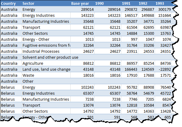
Recently Ken Puls did a handy post on how to unpivot data using PowerQuery. Jan Karel commented that you can do this using Multiple Consolidation Ranges. That’s true, but what I like about the PowerQuery approach is that you can translate the currently selected columns into attribute-value pairs, combined with the rest of the values in each row. That is, you can have multiple hierarchical columns down the left of your CrossTab as well as the column headers across the top that you want to amalgamate. Which is great if you have a crosstab like this:

CrossTab

Whereas the Multiple Consolidation trick only handles one column down the left out of the box.

Mike Alexander posted a great bacon-tasting morsel of a trick to get around that issue way back in 2009 when he used to blog. He simply concatenating all the non-column-oriented fields into one dimension field into one temporary column. Check out his post Transposing a Dataset with a PivotTable. But as commenter dermotb said…it’s like a magic spell that you have to write down somewhere, and try to find when you need it, because it’s complex. (I love Mike’s reply to that: Come on. Excel is full of magic syntax, mystical hot keys, and vba voodoo that requires some level of memorizing steps. That’s why I can make a living peddling “tips and tricks”.)

Another problem with the Multiple Consolidation trick is that you might well end up with more data than fits in your sheet, by the time you flatten it out. Especially in old Excel. Because the number of rows you end up with in a flat file is the number of rows you start off with times the number of columns that you’re going to amalgamate. So for say a time-series dataset that covers quite a few items and a reasonable period of time, you could be in trouble.

So a while ago I had a crack at writing a SQL routine that unpivots by doing lots of UNION ALL joins, and writes the data directly to a PivotTable. The UNION ALLs are required because the pidgin English version of SQL that Excel speaks (and Access too, I guess) doesn’t have a UNPIVOT command.

I struck a few hurdles along the way. For instance, it turns out that the Microsoft JET/ACE Database engine has a hard limit of 50 ‘UNION ALL’ clauses, which you will soon exceed if you have a big crosstab with multiple columns down the left. I found a great thread over at MrExcel at which Fazza overcame this hard limit by creating sub-blocks of UNION ALL statements, then stiching them all together with another UNION ALL. Another problem is that SQL didn’t like dates (and sometimes numbers) in the headers. So I turn them into text with an apostrophe.

And another thing I do is save a temp version of the file somewhere, and then query that temp version rather than querying the open workbook. Even though the Memory Leak issue that this avoids has been largely fixed in New Excel, I still found that querying the open book was causing grief occasionally.

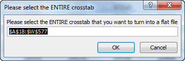
Anyway, here’s the result. I’ve turned it into a function, and you can pre-specify inputs if you like. Otherwise you’ll be prompted for the following:

20131119_UnPivot_Select Entire Crosstab

20131119_UnPivot_Select Left Column Headers

20131119_UnPivot_Select Crosstab Column Headers

20131119_UnPivot_FieldName

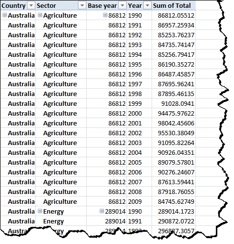
…and then you’ll get a Pivot:

20131119_UnPivot_Output

Take it for a spin, let me know of any issues in the comments. Note that I’ve tried to code it to handle Excel 2003 and earlier, but I don’t have old Excel anymore so couldn’t test it. In fact, that’s why the TabularLayout sub is separate – I had to put it in a subroutine because if someone has ‘old’ Excel then the main function wouldn’t compile.

Cheers

Jeff

Sub CallUnPivotBySQL()
    UnPivotBySQL
End Sub


Function UnPivotBySQL(Optional rngCrosstab As Range, _
                      Optional rngLeftHeaders As Range, _
                      Optional rngRightHeaders As Range, _
                      Optional strCrosstabName As String) As Boolean

'   Description:    Turns a crosstab file into a flatfile (equivalent to the 'UNPIVOT' command in SQL Server)
'                   and makes a pivottable out of it.  Basically it rotates columns of a table-valued expression
'                   into column values. Base code from Fazza at MR EXCEL forum:
'                   http://www.mrexcel.com/forum/showthread.php?315768-Creating-a-pivot-table-with-multiple-sheets


'   Programmer:     Jeff Weir
'   Contact:        weir.jeff@gmail.com or heavydutydata@gmail.com

'   Name/Version:    Date:      Ini:    Modification:
'   UnPivotBySQL V1  20131119   JSW     Original development


'   Inputs:         Range of the entile crosstab
'                   Range of columns down the left that WON'T be normalized
'                   Range of columns down the right that WILL be normalize
'                   String containing the name to give columns that will be normalized

'   Outputs:        A pivottable of the input data on a new worksheet.

'   Example:

'   It takes a crosstabulated table that looks like this:

'   Country        Sector          1990        1991        ...         2009
'   =============================================================================
'   Australia      Energy          290,872     296,887     ...         417,355
'   New Zealand    Energy          23,915      25,738      ...         31,361
'   United States  Energy          5,254,607   5,357,253   ...         5,751,106
'   Australia      Manufacturing   35,648      35,207      ...         44,514
'   New Zealand    Manufacturing   4,389       4,845       ...         4,907
'   United States  Manufacturing   852,424     837,828     ...         735,902
'   Australia      Transport       62,121      61,504      ...         83,645
'   New Zealand    Transport       8,679       8,696       ...         13,783
'   United States  Transport       1,484,909   1,447,234   ...         1,722,501


'   And it returns the same data in a recordset organised like this:

'   Country        Sector          Year        Value
'   ====================================================
'   Australia      Energy          1990        290,872
'   New Zealand    Energy          1990        23,915
'   United States  Energy          1990        5,254,607
'   Australia      Manufacturing   1990        35,648
'   New Zealand    Manufacturing   1990        4,389
'   United States  Manufacturing   1990        852,424
'   Australia      Transport       1990        62,121
'   New Zealand    Transport       1990        8,679
'   United States  Transport       1990        1,484,909
'   Australia      Energy          1991        296,887
'   New Zealand    Energy          1991        25,738
'   United States  Energy          1991        5,357,253
'   Australia      Manufacturing   1991        35,207
'   New Zealand    Manufacturing   1991        4,845
'   United States  Manufacturing   1991        837,828
'   Australia      Transport       1991        61,504
'   New Zealand    Transport       1991        8,696
'   United States  Transport       1991        1,447,234
'   ...            ...             ...         ...
'   ...            ...             ...         ...
'   ...            ...             ...         ...
'   Australia      Energy          2009        417,355
'   New Zealand    Energy          2009        31,361
'   United States  Energy          2009        5,751,106
'   Australia      Manufacturing   2009        44,514
'   New Zealand    Manufacturing   2009        4,907
'   United States  Manufacturing   2009        735,902
'   Australia      Transport       2009        83,645
'   New Zealand    Transport       2009        13,783
'   United States  Transport       2009        1,722,501

'   Base code from Fazza at MR EXCEL:
'   http://www.mrexcel.com/forum/showthread.php?315768-Creating-a-pivot-table-with-multiple-sheets

'   Fazza's code base was perfect for this, given that:
'        A) unwinding a crosstab requires heavy use of 'UNION ALL' in absence of an 'UNPIVOT' command,
'        B) The Microsoft JET/ACE Database engine has a hard limit of 50 'UNION ALL' clauses, but Fazza's
'            code gets around this by creating sublocks of up to 25 SELECT/UNION ALL statements, and
'            then unioning these.
'        C) unwinding a BIG crosstab by using the 'reverse pivot' trick via multiple consolidation ranges
'           might well result in more data that the worksheet can handle.
'

    Const lngMAX_UNIONS As Long = 25

    Dim i As Long, j As Long
    Dim arSQL() As String
    Dim arTemp() As String
    Dim sTempFilePath As String
    Dim objPivotCache As PivotCache
    Dim objRS As Object
    Dim oConn As Object
    Dim sConnection As String
    Dim wksNew As Worksheet
    Dim cell As Range
    Dim strLeftHeaders As String
    Dim wksSource As Worksheet
    Dim pt As PivotTable
    Dim rngCurrentHeader As Range

    Const Success As Boolean = True
    Const Failure As Boolean = False

    UnPivotBySQL = Failure

    If ActiveWorkbook.Path <> "" Then    'can only proceed if the workbook has been saved somewhere

        'Identify where the ENTIRE crosstab table is
        If rngCrosstab Is Nothing Then
            On Error Resume Next
            Set rngCrosstab = Application.InputBox( _
                              Title:="Please select the ENTIRE crosstab", _
                              prompt:="Please select the ENTIRE crosstab that you want to turn into a flat file", _
                              Type:=8, Default:=Selection.CurrentRegion.Address)
            If Err.Number <> 0 Then
                On Error GoTo errhandler
                Err.Raise 999
            Else: On Error GoTo errhandler
            End If
            rngCrosstab.Parent.Activate
            rngCrosstab.Cells(1, 1).Select    'Returns them to the top left of the source table for convenience
        End If

        'Identify range containing columns of interest running down the table
        If rngLeftHeaders Is Nothing Then
            On Error Resume Next
            Set rngLeftHeaders = Application.InputBox( _
                                 Title:="Select the column HEADERS from the LEFT of the table that WON'T be aggregated", _
                                 prompt:="Select the column HEADERS from the LEFT of the table that won't be aggregated", _
                                 Default:=Selection.Address, Type:=8)
            If Err.Number <> 0 Then
                On Error GoTo errhandler
                Err.Raise 999
            Else: On Error GoTo errhandler
            End If
            Set rngLeftHeaders = rngLeftHeaders.Resize(1, rngLeftHeaders.Columns.Count)    'just in case they selected the entire column
            rngLeftHeaders.Cells(1, rngLeftHeaders.Columns.Count + 1).Select    'Returns them to the right of the range they just selected
        End If


        If rngRightHeaders Is Nothing Then
            'Identify range containing data and cross-tab headers running across the table
            On Error Resume Next
            Set rngRightHeaders = Application.InputBox( _
                                  Title:="Select the column HEADERS from the RIGHT of the table that WILL be aggregated", _
                                  prompt:="Select the column HEADERS from the RIGHT of the table that WILL be aggregated", _
                                  Default:=Selection.Address, _
                                  Type:=8)
             If Err.Number <> 0 Then
                On Error GoTo errhandler
                Err.Raise 999
            Else: On Error GoTo errhandler
            End If
            Set rngRightHeaders = rngRightHeaders.Resize(1, rngRightHeaders.Columns.Count)    'just in case they selected the entire column
            rngCrosstab.Cells(1, 1).Select    'Returns them to the top left of the source table for convenience
        End If


        If strCrosstabName = "" Then

            'Get the field name for the columns being consolidated e.g. 'Country' or 'Project'. note that reserved SQL words like 'Date' cannot be used
            strCrosstabName = Application.InputBox( _
                              Title:="What name do you want to give the data field being aggregated?", _
                              prompt:="What name do you want to give the data field being aggregated? e.g. 'Date', 'Country', etc.", _
                              Default:="Date", _
                              Type:=2)
             If strCrosstabName = "False" Then Err.Raise 999

        End If

        Application.ScreenUpdating = False


        Set wksSource = rngLeftHeaders.Parent

        'Build part of SQL Statement that deals with 'static' columns i.e. the ones down the left
        For Each cell In rngLeftHeaders
       
            'For some reason this approach doesn't like columns with numeric headers.
            ' My solution in the below line is to prefix any numeric characters with
            ' an apostrophe to render them non-numeric, and restore them back to numeric
            ' after the query has run
           
            If IsNumeric(cell) Or IsDate(cell) Then cell.Value = "'" & cell.Value
            strLeftHeaders = strLeftHeaders & "[" & cell.Value & "], "
           
        Next cell

        ReDim arTemp(1 To lngMAX_UNIONS)    'currently 25 as per declaration at top of module

        ReDim arSQL(1 To (rngRightHeaders.Count - 1) \ lngMAX_UNIONS + 1)

        For i = LBound(arSQL) To UBound(arSQL) - 1
            For j = LBound(arTemp) To UBound(arTemp)
                Set rngCurrentHeader = rngRightHeaders(1, (i - 1) * lngMAX_UNIONS + j)

                arTemp(j) = "SELECT " & strLeftHeaders & "[" & rngCurrentHeader.Value & "] AS Total, '" & rngCurrentHeader.Value & "' AS [" & strCrosstabName & "] FROM [" & rngCurrentHeader.Parent.Name & "$" & Replace(rngCrosstab.Address, "$", "") & "]"
                If IsNumeric(rngCurrentHeader) Or IsDate(rngCurrentHeader) Then rngCurrentHeader.Value = "'" & rngCurrentHeader.Value    'As per above, can't have numeric headers

            Next j
            arSQL(i) = "(" & Join$(arTemp, vbCr & "UNION ALL ") & ")"
        Next i

        ReDim arTemp(1 To rngRightHeaders.Count - (i - 1) * lngMAX_UNIONS)
        For j = LBound(arTemp) To UBound(arTemp)
            Set rngCurrentHeader = rngRightHeaders(1, (i - 1) * lngMAX_UNIONS + j)
            arTemp(j) = "SELECT " & strLeftHeaders & "[" & rngCurrentHeader.Value & "] AS Total, '" & rngCurrentHeader.Value & "' AS [" & strCrosstabName & "] FROM [" & rngCurrentHeader.Parent.Name & "$" & Replace(rngCrosstab.Address, "$", "") & "]"
            If IsNumeric(rngCurrentHeader) Or IsDate(rngCurrentHeader) Then rngCurrentHeader.Value = "'" & rngCurrentHeader.Value   'As per above, can't have numeric headers

        Next j
        arSQL(i) = "(" & Join$(arTemp, vbCr & "UNION ALL ") & ")"
        'Debug.Print Join$(arSQL, vbCr & "UNION ALL" & vbCr)

        '''''''''''''''''''''''''''''''''''''''''''''''''''''''''''''''''
        ' When using ADO with Excel data, there is a documented bug
        ' causing a memory leak unless the data is in a different
        ' workbook from the ADO workbook.
        ' http://support.microsoft.com/kb/319998
        ' So the work-around is to save a temp version somewhere else,
        ' then pull the data from the temp version, then delete the
        ' temp copy
        sTempFilePath = ActiveWorkbook.Path
        sTempFilePath = sTempFilePath & "\" & "TempFile_" & Format(Time(), "hhmmss") & ".xlsm"
        ActiveWorkbook.SaveCopyAs sTempFilePath
        '''''''''''''''''''''''''''''''''''''''''''''''''''''''''''''''''

         If Application.Version >= 12 Then
            'use ACE provider connection string
           sConnection = "Provider=Microsoft.ACE.OLEDB.12.0; Data Source=" & sTempFilePath & ";Extended Properties=""Excel 12.0;"""
            Else
            'use JET provider connection string
            sConnection = "Provider=Microsoft.Jet.OLEDB.4.0; Data Source=" & sTempFilePath & ";Extended Properties=""Excel 8.0;"""
        End If
       
        Set objRS = CreateObject("ADODB.Recordset")
        Set oConn = CreateObject("ADODB.Connection")
       
        ' Open the ADO connection to our temp Excel workbook
        oConn.Open sConnection
       
         ' Open the recordset as a result of executing the SQL query
        objRS.Open Source:=Join$(arSQL, vbCr & "UNION ALL" & vbCr), ActiveConnection:=oConn, CursorType:=3   'adOpenStatic !!!NOTE!!! we have to use a numerical constant here, because as we are using late binding Excel doesn't have a clue what 'adOpenStatic' means
   
        Set objPivotCache = ActiveWorkbook.PivotCaches.Create(xlExternal)
        Set objPivotCache.Recordset = objRS
        Set objRS = Nothing

        Set wksNew = Sheets.Add
        Set pt = objPivotCache.CreatePivotTable(TableDestination:=wksNew.Range("A3"))
        Set objPivotCache = Nothing

        'Turn any numerical headings back to numbers by effectively removing any apostrophes in front
        For Each cell In rngLeftHeaders
            If IsNumeric(cell) Or IsDate(cell) Then cell.Value = cell.Value
        Next cell
        For Each cell In rngRightHeaders
            If IsNumeric(cell) Or IsDate(cell) Then cell.Value = cell.Value
        Next cell

        With pt
            .ManualUpdate = True    'stops the pt refreshing while we make chages to it.
            If Application.Version >= 14 Then TabularLayout pt
           

            For Each cell In rngLeftHeaders
                With .PivotFields(cell.Value)
                    .Orientation = xlRowField
                    .Subtotals = Array(False, False, False, False, False, False, False, False, False, False, False, False)
                End With
            Next cell

            With .PivotFields(strCrosstabName)
                .Orientation = xlRowField
                .Subtotals = Array(False, False, False, False, False, False, False, False, False, False, False, False)
            End With

            With .PivotFields("Total")
                .Orientation = xlDataField
                .Function = xlSum
            End With
            .ManualUpdate = False
        End With
       
        UnPivotBySQL = Success
    Else: MsgBox "You must first save the workbook for this code to work."
    End If
   
errhandler:
    If Err.Number <> 0 Then
        Select Case Err.Number
            Case 999: 'User pushed cancel.
            Case Else:  MsgBox "Whoops, there was an error: Error#" & Err.Number & vbCrLf & Err.Description _
                     , vbCritical, "Error", Err.HelpFile, Err.HelpContext
        End Select
    End If

Application.ScreenUpdating = True

End Function

Private Sub TabularLayout(pt As PivotTable)
    With pt
        .RepeatAllLabels xlRepeatLabels
        .RowAxisLayout xlTabularRow
    End With
End Sub

In an ideal world

$
0
0

Howdy folks. Jeff here, with yet another post on Pivot Tables.

Just kidding. :-)

My good internet pal Craig Hatmaker gives me a friendly ribbing every time I send him some code that does something in Excel that a database could implement much more efficiently. He points out that because he’s in IT, he doesn’t have anyone stopping him from doing things as he thinks they should be done. So he has no impediment to doing what seems ideal to him.

And he points out that you needn’t be from an IT background in order to replicate his type of approach: if you can master xl, you can master databases. (And he should know: check out his amazing Beyond Excel: VBA and Database Manipulation blog, where he starts off with looking at how to use simple things like Microsoft Query to get data, then progressively teaches you more and more every post until you’re using excel to add records to an access database using a table driven approach, so you don’t have to write SQL or update a single line of code. )

I agree 100%. If you can master xl, you can master databases. The problem is, most people don’t master the first. And out of those that do, many don’t choose to master the second. So the majority will continue to shoehorn large datasets into Excel crosstabs, and then do incredibly convoluted things in order to get the equivalent functionality of a PivotTable out of those crosstabs.

And so I’ll continue to build routines like my Unpivot Via SQL and Filter Pivots Based on External ranges to help them manage their lunacy. Even though I know I shouldn’t encourage them.

This reminds me of the conversation in the comments over at Chandoo’s blog in his post on Speedo Charts called Hack together a Gauge Chart in Excel without sweat, but which Jon Peltier would likely retitle Speedo Charts: The Little Chart That Shouldn’t:

  • Jon Peltier: Speedo charts? Do you really want to encourage such poor presentation techniques
  • Me: Despite the fact that we “shouldn’t really” use dials, I think that if a paying client or monster boss wants them and it’s a deal-breaker, then we best know how to whip one up.
  • Chandoo: As long as we have bosses asking for gauges, we will have gauge charts.
  • Anonymous Reader: Thank you for you posts Chandoo. Gauge/Speedometer chart is exactly what my superiors asked me to make for next EB meeting.
  • Jon: Another happy reader led astray by the gauge chart instructions in this post.
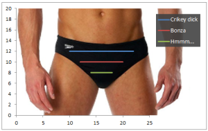
  • Me: Here’s a legitimate speedo chart that I’m sure even Stephen Few couldn’t argue with:
    DDOE_BestPractice_20131121

Explanation for non-Australian or non-New Zealand readers:
Speedos: Gentlemen’s bathing suit, typically in close form-fitting style.
Bonza: Slang for “remarkable or wonderful”
Crikey Dick: expression of surprise

Craig sums this up this tension between utopia and reality really succinctly: “That’s why we work in opposite directions. I do what seems ideal. You do what is necessary given restraints.”

*Sigh*. Afraid so. On the upside, I’ve formulated this into two helpful business rules:

Rule number 1: As long as clients keep shoehorning large amount of data badly in Excel, they will inevitably get into an urgent pickle.
Rule number 2: As long as Rule Number 1 holds true, I will continue to charge an ‘urgent pickle’ hourly rate.

On rule number 1, I’ve told several clients again and again that they need to migrate their 100MB+ spreadsheets to 0.05 MB database tables. I point out that these spreadsheets are inevitably just one in a chain of fat spreadsheets that contain data they use to make up monthly reports for clients. And I highlight that just getting those monthly BAU reports out the door inevitably has become a full-time exercise.
But they won’t migrate this data to a more sensible solution, because:

  1. They don’t know whether the benefit of migration will outweigh the cost, and/or
  2. They don’t want the hassle of working out how to migrate, and/or
  3. They don’t want to master SQL, and/or
  4. I’m really crap at communicating this stuff, and/or
  5. This is the least pressing of their pressing business issues.

On that second point, I point out that their existing process is nothing but hassle, and that it will be a real big hassle when their spreadsheet finally dies, along with all their data. And on point 5, by the time this becomes the most pressing of their pressing business issues, they no longer have a business.

On that 3rd point, they generally answer “we are Economists/Accountants/Whatevers, not Data Analysts”. I say “Given your business is built around data, you are Data Analysts first, and Whatevers second”.
Cue blank stare.
*Sigh*


UnPivot Shootout

$
0
0

Jeff here, again. PivotTables again. Sorry ’bout that.

snb posted a very concise bit of code to unwind crosstabs over at Unpivot by SQL and so I got to wondering how my much longer routine handled in comparison.

My approach used SQL and lots of Union All statements to do the trick. And lots and lots of code. Whereas snb uses arrays to unwind the crosstab, which is fine so long as you don’t run out of worksheet to post the resulting flat-file in. Which is going to be the case 99.999999% of the time. And frankly, crosstabs in the other 0.000001% of cases deserve to be stuck as crosstabs.

At the same time, I thought I’d also test a previous approach of mine that uses the Multiple Consolidation trick that Mike Alexander outlines at Transposing a Dataset with a PivotTable. This approach:

  1. copies the specific contiguous or non-contiguous columns of data that the user want to turn into a flat file to a new sheet.
  2. concatenates all the columns on the left into one column, while putting the pipe character ‘|’ between each field so that later we can split these apart into separate columns again.
  3. creates a pivot table out of this using Excel’s ‘Multiple Consolidation Ranges’ option. Normally this type of pivot table is used for combining data on different sheets, but it has the side benefit of taking horizontal data and providing a vertical extract once you double click on the Grand Total field. This is also known as a ‘Reverse Pivot’.
  4. splits our pipe-delimited column back into seperate columns, using Excel’s Text-to-Column funcionality.

snb’s approach

snbs’ code for a dataset with two non-pivot fields down the left looked like this:

Sub M_snb()
    sn = Cells(1).CurrentRegion
    x = Cells(1).CurrentRegion.Rows(1).SpecialCells(2).Count
    y = UBound(sn, 2) - x
   
    ReDim sp(1 To x * (UBound(sn) - 1), 1 To 4)
   
    For j = 1 To UBound(sp)
       m = (j - 1) Mod (UBound(sn) - 1) + 2
       n = (j - 1) \ (UBound(sn) - 1) + y + 1
       sp(j, 1) = sn(m, 1)
       sp(j, 2) = sn(m, 2)
       sp(j, 3) = sn(1, n)
       sp(j, 4) = sn(m, n)
    Next
   
    Cells(20, 1).Resize(UBound(sp), UBound(sp, 2)) = sp
End Sub

…which I’m sure you’ll all agree falls somewhere on the spectrum between good looking and positivity anorexic. So I put a bit of meat on it’s bones so that it prompts you for ranges and handles any sized cross-tab:

Sub UnPivot_snb()
    Dim varSource As Variant
    Dim j As Long
    Dim m As Long
    Dim n As Long
    Dim i As Long
    Dim varOutput As Variant
    Dim rngCrossTab As Range
    Dim rngLeftHeaders As Range
    Dim rngRightHeaders As Range
   
'Identify where the ENTIRE crosstab table is
        If rngCrossTab Is Nothing Then
            On Error Resume Next
            Set rngCrossTab = Application.InputBox( _
                              Title:="Please select the ENTIRE crosstab", _
                              prompt:="Please select the ENTIRE crosstab that you want to turn into a flat file", _
                              Type:=8, Default:=Selection.CurrentRegion.Address)
            If Err.Number <> 0 Then
                On Error GoTo errhandler
                Err.Raise 999
            Else: On Error GoTo errhandler
            End If
            rngCrossTab.Parent.Activate
            rngCrossTab.Cells(1, 1).Select    'Returns them to the top left of the source table for convenience
        End If

        'Identify range containing columns of interest running down the table
        If rngLeftHeaders Is Nothing Then
            On Error Resume Next
            Set rngLeftHeaders = Application.InputBox( _
                                 Title:="Select the column HEADERS from the LEFT of the table that WON'T be aggregated", _
                                 prompt:="Select the column HEADERS from the LEFT of the table that won't be aggregated", _
                                 Default:=Selection.Address, Type:=8)
            If Err.Number <> 0 Then
                On Error GoTo errhandler
                Err.Raise 999
            Else: On Error GoTo errhandler
            End If
            Set rngLeftHeaders = rngLeftHeaders.Resize(1, rngLeftHeaders.Columns.Count)    'just in case they selected the entire column
            rngLeftHeaders.Cells(1, rngLeftHeaders.Columns.Count + 1).Select    'Returns them to the right of the range they just selected
        End If


        If rngRightHeaders Is Nothing Then
            'Identify range containing data and cross-tab headers running across the table
            On Error Resume Next
            Set rngRightHeaders = Application.InputBox( _
                                  Title:="Select the column HEADERS from the RIGHT of the table that WILL be aggregated", _
                                  prompt:="Select the column HEADERS from the RIGHT of the table that WILL be aggregated", _
                                  Default:=Selection.Address, _
                                  Type:=8)
             If Err.Number <> 0 Then
                On Error GoTo errhandler
                Err.Raise 999
            Else: On Error GoTo errhandler
            End If
            Set rngRightHeaders = rngRightHeaders.Resize(1, rngRightHeaders.Columns.Count)    'just in case they selected the entire column
            rngCrossTab.Cells(1, 1).Select    'Returns them to the top left of the source table for convenience
        End If


        If strCrosstabName = "" Then
            'Get the field name for the columns being consolidated e.g. 'Country' or 'Project'. note that reserved SQL words like 'Date' cannot be used
            strCrosstabName = Application.InputBox( _
                              Title:="What name do you want to give the data field being aggregated?", _
                              prompt:="What name do you want to give the data field being aggregated? e.g. 'Date', 'Country', etc.", _
                              Default:="Date", _
                              Type:=2)
             If strCrosstabName = "False" Then Err.Raise 999
        End If

    timetaken = Now()

    varSource = rngCrossTab
    lRightColumns = rngRightHeaders.Columns.Count
    lLeftColumns = UBound(varSource, 2) - lRightColumns
   
    ReDim varOutput(1 To lRightColumns * (UBound(varSource) - 1), 1 To lLeftColumns + 2)
   
    For j = 1 To UBound(varOutput)
        m = (j - 1) Mod (UBound(varSource) - 1) + 2
        n = (j - 1) \ (UBound(varSource) - 1) + lLeftColumns + 1
        varOutput(j, lLeftColumns + 1) = varSource(1, n)
        varOutput(j, lLeftColumns + 2) = varSource(m, n)
        For i = 1 To lLeftColumns
            varOutput(j, i) = varSource(m, i)
        Next i
    Next j
   
    Worksheets.Add

    With Cells(1, 1)
        .Resize(, lLeftColumns).Value = rngLeftHeaders.Value
        .Offset(, lLeftColumns).Value = strCrosstabName
        .Offset(, lLeftColumns + 1).Value = "Value"
        .Offset(1, 0).Resize(UBound(varOutput), UBound(varOutput, 2)) = varOutput
    End With
   
   
timetaken = timetaken - Now()
   
    Debug.Print "UnPivot - snb: " & Now() & " Time Taken: " & Format(timetaken, "HH:MM:SS")
errhandler:
    If Err.Number <> 0 Then
        Dim strErrMsg As String
        Select Case Err.Number
        Case 999: 'User pushed cancel. Do nothing
        Case 998   'Worksheet does not have enough rows to hold flat file
            strErrMsg = "Oops, there's not enough rows in the worsheet to hold a flatfile of all the data you have selected. "
            strErrMsg = strErrMsg & vbNewLine & vbNewLine
            strErrMsg = strErrMsg & "Your dataset will take up " & Format(rngRightHeaders.CurrentRegion.Count, "#,##0") & " rows of data "
            strErrMsg = strErrMsg & "but your worksheet only allows " & Format(Application.Range("A:A").Count, "#,##0") & " rows of data. "
            strErrMsg = strErrMsg & vbNewLine & vbNewLine
            MsgBox strErrMsg

        Case Else
            MsgBox Err.Description, vbCritical, "UnPivot_snb"

        End Select

    End If
End Sub

Talk about yo-yo dieting!

Multiple Consolidation Trick approach

And here’s my code that uses the Multiple Consolidation trick:

Option Explicit

Sub CallUnPivotByConsolidation()
Call UnPivotByConsolidation
End Sub

Function UnPivotByConsolidation( _
                      Optional rngCrossTab As Range, _
                      Optional rngLeftHeaders As Range, _
                      Optional rngRightHeaders As Range, _
                      Optional strCrosstabName As String) As Boolean

    Dim wksTempCrosstab As Worksheet
    Dim wksInitial As Worksheet
    Dim strConcat As String
    Dim strCell As String
    Dim strFormula As String
    Dim iCount As Integer
    Dim iColumns As Integer
    Dim iRows As Integer
    Dim rngInputData As Range
    Dim wksPT As Worksheet
    Dim wksFlatFile As Worksheet
    Dim pc As PivotCache
    Dim pt As PivotTable
    Dim rngKeyFormula As Range
    Dim rngRowHeaders As Range
    Dim rngPT_GrandTotal As Range, rngPTData As Range
    Dim lPT_Rows As Long
    Dim iPT_Columns As Integer
    Dim iKeyColumns As Integer
    Dim varRowHeadings  As Variant


    '''''''''''''''''''''''''''''''''''''''''''''''''''''''''''''''''''''''''''''
    'Part one:                                                                  '
    'Code prompts user to select contiguous or non-contiguous columns of data   '
    'from a crosstab table, and writes it to a new sheet in a contiguous range. '
    '''''''''''''''''''''''''''''''''''''''''''''''''''''''''''''''''''''''''''''

    Set wksInitial = ActiveSheet


'Identify where the ENTIRE crosstab table is
    If rngCrossTab Is Nothing Then
        On Error Resume Next
        Set rngCrossTab = Application.InputBox( _
                          Title:="Please select the ENTIRE crosstab", _
                          prompt:="Please select the ENTIRE crosstab that you want to turn into a flat file", _
                          Type:=8, Default:=Selection.CurrentRegion.Address)
        If Err.Number <> 0 Then
            On Error GoTo errhandler
            Err.Raise 999
        Else: On Error GoTo errhandler
        End If
        rngCrossTab.Parent.Activate
        rngCrossTab.Cells(1, 1).Select    'Returns them to the top left of the source table for convenience
    End If


'Identify range containing columns of interest running down the table
    If rngLeftHeaders Is Nothing Then
        On Error Resume Next
        Set rngLeftHeaders = Application.InputBox( _
                             Title:="Select the column HEADERS from the LEFT of the table that WON'T be aggregated", _
                             prompt:="Select the column HEADERS from the LEFT of the table that won't be aggregated", _
                             Default:=Selection.Address, Type:=8)
        If Err.Number <> 0 Then
            On Error GoTo errhandler
            Err.Raise 999
        Else: On Error GoTo errhandler
        End If
        Set rngLeftHeaders = Intersect(rngLeftHeaders.EntireColumn, rngCrossTab)
        rngLeftHeaders.Cells(1, rngLeftHeaders.Columns.Count + 1).Select    'Returns them to the right of the range they just selected
    End If
   
    If rngRightHeaders Is Nothing Then
        'Identify range containing data and cross-tab headers running across the table
        On Error Resume Next
        Set rngRightHeaders = Application.InputBox( _
                              Title:="Select the column HEADERS from the RIGHT of the table that WILL be aggregated", _
                              prompt:="Select the column HEADERS from the RIGHT of the table that WILL be aggregated", _
                              Default:=Selection.Address, _
                              Type:=8)
         If Err.Number <> 0 Then
            On Error GoTo errhandler
            Err.Raise 999
        Else: On Error GoTo errhandler
        End If
        Set rngRightHeaders = Intersect(rngRightHeaders.EntireColumn, rngCrossTab)
        rngCrossTab.Cells(1, 1).Select    'Returns them to the top left of the source table for convenience
    End If

    If strCrosstabName = "" Then
        'Get the field name for the columns being consolidated e.g. 'Country' or 'Project'. note that reserved SQL words like 'Date' cannot be used
        strCrosstabName = Application.InputBox( _
                          Title:="What name do you want to give the data field being aggregated?", _
                          prompt:="What name do you want to give the data field being aggregated? e.g. 'Date', 'Country', etc.", _
                          Default:="Date", _
                          Type:=2)
         If strCrosstabName = "False" Then Err.Raise 999
    End If
   
    With Application
        .ScreenUpdating = False
        .DisplayAlerts = False
    End With
   
     'Set up a temp worksheet to house our crosstab data
    For Each wksTempCrosstab In ActiveWorkbook.Worksheets
        If wksTempCrosstab.Name = "TempCrosstab" Then wksTempCrosstab.Delete
    Next
    Set wksTempCrosstab = Worksheets.Add
    wksTempCrosstab.Name = "TempCrosstab"

    'Copy data to the temp worksheet "TempCrosstab"
    rngLeftHeaders.Copy wksTempCrosstab.[A1]
    Set rngLeftHeaders = wksTempCrosstab.[A1].CurrentRegion
    rngLeftHeaders.Name = "TempCrosstab!appRowFields"
    rngRightHeaders.Copy wksTempCrosstab.[A1].Offset(0, rngLeftHeaders.Columns.Count)
    Set rngRightHeaders = wksTempCrosstab.[A1].Resize(rngRightHeaders.Rows.Count, rngRightHeaders.Columns.Count)
    rngRightHeaders.Name = "TempCrosstab!appCrosstabFields"

    'Work out if the worksheet has enough rows to fit a crosstab in
    If rngRightHeaders.CurrentRegion.Count > Columns(1).Rows.Count Then Err.Raise 998

    varRowHeadings = rngLeftHeaders.Value

    '''''''''''''''''''''''''''''''''''''''''''''''''''''''''''''''''''''''''''''
    'Part Two:                                                                  '
    'Construct a new pipe-delimited column out of the columns that run down the '
    'left of the crosstab, and then delete the original columns used to do this '
    '''''''''''''''''''''''''''''''''''''''''''''''''''''''''''''''''''''''''''''

    strFormula = "=RC[1]"
    strConcat = "&""|""&"

    iColumns = Range("TempCrosstab!appRowFields").Columns.Count

    For iCount = 2 To iColumns
        strCell = "RC[" & iCount & "]"
        strFormula = strFormula & strConcat & strCell
    Next iCount

    With Worksheets("TempCrosstab")
        .Columns("A:A").Insert Shift:=xlToRight
        iRows = Intersect(Worksheets("TempCrosstab").Columns(2), Worksheets("TempCrosstab").UsedRange).Rows.Count
        .Range("A2:A" & iRows).FormulaR1C1 = strFormula
        .Range("A2:A" & iRows).Value = .Range("A2:A" & iRows).Value
        .Range("appRowFields").Delete Shift:=xlToLeft
    End With

    Names("TempCrosstab!appRowFields").Delete

    '''''''''''''''''''''''''''''''''''''''''''''''''''''''''''''''''''''''''''''''''
    'Part Three:                                                                    '
    'Use data to create a pivot table using "Multiple Consolidation Ranges" option, '
    'which has the side benefit of providing a vertical extract once you double     '
    'click on the Grand Total field                                                 '
    '''''''''''''''''''''''''''''''''''''''''''''''''''''''''''''''''''''''''''''''''
    Set rngInputData = Worksheets("TempCrosstab").[A2].CurrentRegion
    rngInputData.Name = "SourceData"

    'Find out the number of columns contained within the primary key
    iKeyColumns = Len([SourceData].Cells(2, 1).Value) - Len(Replace([SourceData].Cells(2, 1).Value, "|", "")) + 1

    '   Create the intermediate pivot from which to extract flat file
    Set pc = ActiveWorkbook.PivotCaches.Add(SourceType:=xlConsolidation, SourceData:=Array("=sourcedata", "Item1"))
    Set wksPT = Worksheets.Add
    Set pt = wksPT.PivotTables.Add(PivotCache:=pc, TableDestination:=[A3])


    '   Get address of PT Total field, then double click it to get underlying records
    Set rngPTData = pt.DataBodyRange
    lPT_Rows = rngPTData.Rows.Count
    iPT_Columns = rngPTData.Columns.Count
    Set rngPT_GrandTotal = rngPTData.Cells(1).Offset(lPT_Rows - 1, iPT_Columns - 1)
    rngPTData.Cells(1).Offset(lPT_Rows - 1, iPT_Columns - 1).Select
    Selection.ShowDetail = True
    Set wksFlatFile = ActiveSheet

    '   Delete current "Flat_File" worksheet if it exists, name current sheet "Flat_File"
    On Error Resume Next
    Sheets("Flat_File").Delete
    On Error GoTo 0
    wksFlatFile.Name = "Flat_File"

    '   Delete unneeded column and the now-unneeded TempCrosstab and wksPT worksheets
    Columns(4).Delete Shift:=xlToLeft
    wksPT.Delete
    Worksheets("TempCrosstab").Delete

    ''''''''''''''''''''''''''''''''''''''''''''''''''''''''''''''''''''''''''''
    'Part Four:                                                                '
    'split our pipe-delimited column back into seperate columns, using Excel's '
    'Text-to-Column funcionality.                                              '
    ''''''''''''''''''''''''''''''''''''''''''''''''''''''''''''''''''''''''''''

    Set rngKeyFormula = Worksheets("Flat_File").Range("A2")
    rngKeyFormula.Name = "appKeyFormula"

    'Find out the number of columns contained within the primary key
    iKeyColumns = Len([appKeyFormula].Cells(2, 1).Value) - Len(Replace([appKeyFormula].Cells(2, 1).Value, "|", "")) + 1

    'Insert columns to the left that we will unpack the Unique Key to
    [B1].Resize(, iKeyColumns).EntireColumn.Insert


    'Split the Unique Key column into its constituent parts,
    'using Excel's Text-to-Columns functionality
    Worksheets("Flat_File").Columns("A:A").Select
    Selection.TextToColumns Destination:=Range("b1"), DataType:=xlDelimited, _
                            ConsecutiveDelimiter:=False, Other:=True, OtherChar:="|"

    'Delete old composite key, add original column headers
    [A1].EntireColumn.Delete
    Set rngRowHeaders = [A1].Resize(1, iKeyColumns)
    rngRowHeaders.Value = varRowHeadings

    'Add new column header with crosstab data name
    [A1].Offset(0, iKeyColumns).Value = strCrosstabName
    Selection.CurrentRegion.Columns.AutoFit
   
    Worksheets("Flat_File").Select

errhandler:
    If Err.Number <> 0 Then
        Dim strErrMsg As String
        Select Case Err.Number
        Case 999: 'User pushed cancel. Do nothing
        Case 998   'Worksheet does not have enough rows to hold flat file
            strErrMsg = "Oops, there's not enough rows in the worsheet to hold a flatfile of all the data you have selected. "
            strErrMsg = strErrMsg & vbNewLine & vbNewLine
            strErrMsg = strErrMsg & "Your dataset will take up " & Format(rngRightHeaders.CurrentRegion.Count, "#,##0") & " rows of data "
            strErrMsg = strErrMsg & "but your worksheet only allows " & Format(Application.Range("A:A").Count, "#,##0") & " rows of data. "
            strErrMsg = strErrMsg & vbNewLine & vbNewLine
            MsgBox strErrMsg

        Case Else
            MsgBox Err.Description, vbCritical, "UnPivotByConsolidation"

        End Select

    End If

With Application
        .ScreenUpdating = True
        .DisplayAlerts = True
    End With
End Function

The SQL appoach is the same as I published here.

And the winner is…

…snb. By a long shot. With the ever-so-slight caveat that you’re crosstabs are not so stupidly fat that the resulting flat file exceeds the number of rows in Excel.

Here’s how things stacked up on a 53 Column x 2146 Row crosstab, which gives a 117,738 row flat-file:

Approach Time (M:SS)
snb 0:01
UnPivotByConsolidation 0:04
UnPivotBySQL 0:14

 
And here’s how things stacked up on a 53 Columns x 19,780 Row crosstab, giving a 1,048,340 row flat-file (i.e. practically the biggest sized crosstab that you can unwind):

Approach Time (M:SS)
snb 0:19
UnPivotByConsolidation 0:42
UnPivotBySQL 2:17

 
So there you have it. Use snb’s code. Unless you have no choice but to use my longer, slower SQL approach.

If you don’t want the hassle of working out which to use, here’s a routine that uses snb’s if possible, and otherwise uses mine:

Option Explicit
Sub Call_UnPivot()
UnPivot
End Sub


Function UnPivot(Optional rngCrossTab As Range, _
                      Optional rngLeftHeaders As Range, _
                      Optional rngRightHeaders As Range, _
                      Optional strCrosstabName As String) As Boolean

'   Desc:   Turns a crosstab file into a flatfile using array manipulation.
'           If the resulting flat file will be too long to fit in the worksheet,
'           the routine uses SQL and lots of 'UNION ALL' statements to do the
'           equivalent of the 'UNPIVOT' command in SQL Server (which is not available
'           in Excel)and writes the result directly to a PivotTable

'           Base code for the SQL UnPivot devived from from Fazza at MR EXCEL forum:
'           http://www.mrexcel.com/forum/showthread.php?315768-Creating-a-pivot-table-with-multiple-sheets
'           The Microsoft JET/ACE Database engine has a hard limit of 50 'UNION ALL' clauses, but Fazza's
'           code gets around this by creating sublocks of up to 25 SELECT/UNION ALL statements, and
'           then unioning these.


'   Programmer:     Jeff Weir
'   Contact:        weir.jeff@gmail.com

'   Name/Version:    Date:      Ini:    Modification:
'   UnPivot V1      20131122    JSW     Original Development
   

'   Inputs:         Range of the entile crosstab
'                   Range of columns down the left that WON'T be normalized
'                   Range of columns down the right that WILL be normalize
'                   String containing the name to give columns that will be normalized

'   Outputs:        A pivottable of the input data on a new worksheet.

'   Example:

'   It takes a crosstabulated table that looks like this:

'   Country        Sector          1990        1991        ...         2009
'   =============================================================================
'   Australia      Energy          290,872     296,887     ...         417,355
'   New Zealand    Energy          23,915      25,738      ...         31,361
'   United States  Energy          5,254,607   5,357,253   ...         5,751,106
'   Australia      Manufacturing   35,648      35,207      ...         44,514
'   New Zealand    Manufacturing   4,389       4,845       ...         4,907
'   United States  Manufacturing   852,424     837,828     ...         735,902
'   Australia      Transport       62,121      61,504      ...         83,645
'   New Zealand    Transport       8,679       8,696       ...         13,783
'   United States  Transport       1,484,909   1,447,234   ...         1,722,501


'   And it returns the same data in a recordset organised like this:

'   Country        Sector          Year        Value
'   ====================================================
'   Australia      Energy          1990        290,872
'   New Zealand    Energy          1990        23,915
'   United States  Energy          1990        5,254,607
'   Australia      Manufacturing   1990        35,648
'   New Zealand    Manufacturing   1990        4,389
'   United States  Manufacturing   1990        852,424
'   Australia      Transport       1990        62,121
'   New Zealand    Transport       1990        8,679
'   United States  Transport       1990        1,484,909
'   Australia      Energy          1991        296,887
'   New Zealand    Energy          1991        25,738
'   United States  Energy          1991        5,357,253
'   Australia      Manufacturing   1991        35,207
'   New Zealand    Manufacturing   1991        4,845
'   United States  Manufacturing   1991        837,828
'   Australia      Transport       1991        61,504
'   New Zealand    Transport       1991        8,696
'   United States  Transport       1991        1,447,234
'   ...            ...             ...         ...
'   ...            ...             ...         ...
'   ...            ...             ...         ...
'   Australia      Energy          2009        417,355
'   New Zealand    Energy          2009        31,361
'   United States  Energy          2009        5,751,106
'   Australia      Manufacturing   2009        44,514
'   New Zealand    Manufacturing   2009        4,907
'   United States  Manufacturing   2009        735,902
'   Australia      Transport       2009        83,645
'   New Zealand    Transport       2009        13,783
'   United States  Transport       2009        1,722,501


    Const lngMAX_UNIONS As Long = 25

    Dim varSource As Variant
    Dim varOutput As Variant
    Dim lLeftColumns As Long
    Dim lRightColumns As Long
    Dim i As Long
    Dim j As Long
    Dim m As Long
    Dim n As Long
    Dim arSQL() As String
    Dim arTemp() As String
    Dim sTempFilePath As String
    Dim objPivotCache As PivotCache
    Dim objRS As Object
    Dim oConn As Object
    Dim sConnection As String
    Dim wksNew As Worksheet
    Dim cell As Range
    Dim strLeftHeaders As String
    Dim wksSource As Worksheet
    Dim pt As PivotTable
    Dim rngCurrentHeader As Range
    Dim timetaken As Date
    Dim strMsg As String
    Dim varAnswer As Variant

    Const Success As Boolean = True
    Const Failure As Boolean = False

    UnPivot = Failure

    'Identify where the ENTIRE crosstab table is
    If rngCrossTab Is Nothing Then
        On Error Resume Next
        Set rngCrossTab = Application.InputBox( _
                          Title:="Please select the ENTIRE crosstab", _
                          prompt:="Please select the ENTIRE crosstab that you want to turn into a flat file", _
                          Type:=8, Default:=Selection.CurrentRegion.Address)
        If Err.Number <> 0 Then
            On Error GoTo errhandler
            Err.Raise 999
        Else: On Error GoTo errhandler
        End If
        rngCrossTab.Parent.Activate
        rngCrossTab.Cells(1, 1).Select    'Returns them to the top left of the source table for convenience
    End If

    'Identify range containing columns of interest running down the table
    If rngLeftHeaders Is Nothing Then
        On Error Resume Next
        Set rngLeftHeaders = Application.InputBox( _
                             Title:="Select the column HEADERS from the LEFT of the table that WON'T be aggregated", _
                             prompt:="Select the column HEADERS from the LEFT of the table that won't be aggregated", _
                             Default:=Selection.Address, Type:=8)
        If Err.Number <> 0 Then
            On Error GoTo errhandler
            Err.Raise 999
        Else: On Error GoTo errhandler
        End If
        Set rngLeftHeaders = rngLeftHeaders.Resize(1, rngLeftHeaders.Columns.Count)    'just in case they selected the entire column
        rngLeftHeaders.Cells(1, rngLeftHeaders.Columns.Count + 1).Select    'Returns them to the right of the range they just selected
    End If


    If rngRightHeaders Is Nothing Then
        'Identify range containing data and cross-tab headers running across the table
        On Error Resume Next
        Set rngRightHeaders = Application.InputBox( _
                              Title:="Select the column HEADERS from the RIGHT of the table that WILL be aggregated", _
                              prompt:="Select the column HEADERS from the RIGHT of the table that WILL be aggregated", _
                              Default:=Selection.Address, _
                              Type:=8)
         If Err.Number <> 0 Then
            On Error GoTo errhandler
            Err.Raise 999
        Else: On Error GoTo errhandler
        End If
        Set rngRightHeaders = rngRightHeaders.Resize(1, rngRightHeaders.Columns.Count)    'just in case they selected the entire column
        rngCrossTab.Cells(1, 1).Select    'Returns them to the top left of the source table for convenience
    End If


    If strCrosstabName = "" Then

        'Get the field name for the columns being consolidated e.g. 'Country' or 'Project'. note that reserved SQL words like 'Date' cannot be used
        strCrosstabName = Application.InputBox( _
                          Title:="What name do you want to give the data field being aggregated?", _
                          prompt:="What name do you want to give the data field being aggregated? e.g. 'Date', 'Country', etc.", _
                          Default:="Date", _
                          Type:=2)
         If strCrosstabName = "False" Then Err.Raise 999

    End If

    timetaken = Now()
    Application.ScreenUpdating = False
       
    'Work out if the worksheet has enough rows to fit a crosstab in
    If Intersect(rngRightHeaders.EntireColumn, rngCrossTab).Cells.Count <= Columns(1).Rows.Count Then
        'Resulting flat file will fit on the sheet, so use array manipulation.
        varSource = rngCrossTab
        lRightColumns = rngRightHeaders.Columns.Count
        lLeftColumns = UBound(varSource, 2) - lRightColumns
       
        ReDim varOutput(1 To lRightColumns * (UBound(varSource) - 1), 1 To lLeftColumns + 2)
       
        For j = 1 To UBound(varOutput)
            m = (j - 1) Mod (UBound(varSource) - 1) + 2
            n = (j - 1) \ (UBound(varSource) - 1) + lLeftColumns + 1
            varOutput(j, lLeftColumns + 1) = varSource(1, n)
            varOutput(j, lLeftColumns + 2) = varSource(m, n)
            For i = 1 To lLeftColumns
                varOutput(j, i) = varSource(m, i)
            Next i
        Next j
       
        Worksheets.Add
   
        With Cells(1, 1)
            .Resize(, lLeftColumns).Value = rngLeftHeaders.Value
            .Offset(, lLeftColumns).Value = strCrosstabName
            .Offset(, lLeftColumns + 1).Value = "Value"
            .Offset(1, 0).Resize(UBound(varOutput), UBound(varOutput, 2)) = varOutput
        End With
           
    Else 'Resulting flat file will fit on the sheet, so use SQL and write result directly to a pivot
        strMsg = " I can't turn this crosstab into a flat file, because the crosstab is so large that"
        strMsg = strMsg & " the resulting flat file will be too big to fit in a worksheet. "
        strMsg = strMsg & vbNewLine & vbNewLine
        strMsg = strMsg & " However, I can still turn this information directly into a PivotTable if you want."
        strMsg = strMsg & " Note that this might take several minutes. Do you wish to proceed?"
        varAnswer = MsgBox(prompt:=strMsg, Buttons:=vbOK + vbCancel + vbCritical, Title:="Crosstab too large!")
        If varAnswer <> 1 Then Err.Raise 999

        If ActiveWorkbook.Path <> "" Then    'can only proceed if the workbook has been saved somewhere
            Set wksSource = rngLeftHeaders.Parent
   
            'Build part of SQL Statement that deals with 'static' columns i.e. the ones down the left
            For Each cell In rngLeftHeaders
           
                'For some reason this approach doesn't like columns with numeric headers.
                ' My solution in the below line is to prefix any numeric characters with
                ' an apostrophe to render them non-numeric, and restore them back to numeric
                ' after the query has run
               
                If IsNumeric(cell) Or IsDate(cell) Then cell.Value = "'" & cell.Value
                strLeftHeaders = strLeftHeaders & "[" & cell.Value & "], "
               
            Next cell
   
            ReDim arTemp(1 To lngMAX_UNIONS)    'currently 25 as per declaration at top of module
   
            ReDim arSQL(1 To (rngRightHeaders.Count - 1) \ lngMAX_UNIONS + 1)
   
            For i = LBound(arSQL) To UBound(arSQL) - 1
                For j = LBound(arTemp) To UBound(arTemp)
                    Set rngCurrentHeader = rngRightHeaders(1, (i - 1) * lngMAX_UNIONS + j)
   
                    arTemp(j) = "SELECT " & strLeftHeaders & "[" & rngCurrentHeader.Value & "] AS Total, '" & rngCurrentHeader.Value & "' AS [" & strCrosstabName & "] FROM [" & rngCurrentHeader.Parent.Name & "$" & Replace(rngCrossTab.Address, "$", "") & "]"
                    If IsNumeric(rngCurrentHeader) Or IsDate(rngCurrentHeader) Then rngCurrentHeader.Value = "'" & rngCurrentHeader.Value    'As per above, can't have numeric headers
   
                Next j
                arSQL(i) = "(" & Join$(arTemp, vbCr & "UNION ALL ") & ")"
            Next i
   
            ReDim arTemp(1 To rngRightHeaders.Count - (i - 1) * lngMAX_UNIONS)
            For j = LBound(arTemp) To UBound(arTemp)
                Set rngCurrentHeader = rngRightHeaders(1, (i - 1) * lngMAX_UNIONS + j)
                arTemp(j) = "SELECT " & strLeftHeaders & "[" & rngCurrentHeader.Value & "] AS Total, '" & rngCurrentHeader.Value & "' AS [" & strCrosstabName & "] FROM [" & rngCurrentHeader.Parent.Name & "$" & Replace(rngCrossTab.Address, "$", "") & "]"
                If IsNumeric(rngCurrentHeader) Or IsDate(rngCurrentHeader) Then rngCurrentHeader.Value = "'" & rngCurrentHeader.Value   'As per above, can't have numeric headers
   
            Next j
            arSQL(i) = "(" & Join$(arTemp, vbCr & "UNION ALL ") & ")"
            'Debug.Print Join$(arSQL, vbCr & "UNION ALL" & vbCr)
   
            '''''''''''''''''''''''''''''''''''''''''''''''''''''''''''''''''
            ' When using ADO with Excel data, there is a documented bug
            ' causing a memory leak unless the data is in a different
            ' workbook from the ADO workbook.
            ' http://support.microsoft.com/kb/319998
            ' So the work-around is to save a temp version somewhere else,
            ' then pull the data from the temp version, then delete the
            ' temp copy
            sTempFilePath = ActiveWorkbook.Path
            sTempFilePath = sTempFilePath & "\" & "TempFile_" & Format(time(), "hhmmss") & ".xlsm"
            ActiveWorkbook.SaveCopyAs sTempFilePath
            '''''''''''''''''''''''''''''''''''''''''''''''''''''''''''''''''
   
             If Application.Version >= 12 Then
                'use ACE provider connection string
               sConnection = "Provider=Microsoft.ACE.OLEDB.12.0; Data Source=" & sTempFilePath & ";Extended Properties=""Excel 12.0;"""
                Else
                'use JET provider connection string
                sConnection = "Provider=Microsoft.Jet.OLEDB.4.0; Data Source=" & sTempFilePath & ";Extended Properties=""Excel 8.0;"""
            End If
           
            Set objRS = CreateObject("ADODB.Recordset")
            Set oConn = CreateObject("ADODB.Connection")
           
            ' Open the ADO connection to our temp Excel workbook
            oConn.Open sConnection
           
             ' Open the recordset as a result of executing the SQL query
            objRS.Open Source:=Join$(arSQL, vbCr & "UNION ALL" & vbCr), ActiveConnection:=oConn, CursorType:=3   'adOpenStatic !!!NOTE!!! we have to use a numerical constant here, because as we are using late binding Excel doesn't have a clue what 'adOpenStatic' means
       
            Set objPivotCache = ActiveWorkbook.PivotCaches.Create(xlExternal)
            Set objPivotCache.Recordset = objRS
            Set objRS = Nothing
   
            Set wksNew = Sheets.Add
            Set pt = objPivotCache.CreatePivotTable(TableDestination:=wksNew.Range("A3"))
            Set objPivotCache = Nothing
   
            'Turn any numerical headings back to numbers by effectively removing any apostrophes in front
            For Each cell In rngLeftHeaders
                If IsNumeric(cell) Or IsDate(cell) Then cell.Value = cell.Value
            Next cell
            For Each cell In rngRightHeaders
                If IsNumeric(cell) Or IsDate(cell) Then cell.Value = cell.Value
            Next cell
   
            With pt
                .ManualUpdate = True    'stops the pt refreshing while we make chages to it.
                If Application.Version >= 14 Then TabularLayout pt
               
   
                For Each cell In rngLeftHeaders
                    With .PivotFields(cell.Value)
                        .Subtotals = Array(False, False, False, False, False, False, False, False, False, False, False, False)
                    End With
                Next cell
   
                With .PivotFields(strCrosstabName)
                    .Subtotals = Array(False, False, False, False, False, False, False, False, False, False, False, False)
                End With
   
                With .PivotFields("Total")
                    .Orientation = xlDataField
                    .Function = xlSum
                End With
                .ManualUpdate = False
            End With
            Else: MsgBox "You must first save the workbook for this code to work."
        End If
    End If
       
    UnPivot = Success
       
    timetaken = timetaken - Now()
    Debug.Print "UnPivot: " & Now() & " Time Taken: " & Format(timetaken, "HH:MM:SS")
       
   
errhandler:
    If Err.Number <> 0 Then
        Select Case Err.Number
            Case 999: 'User pushed cancel.
            Case Else:  MsgBox "Whoops, there was an error: Error#" & Err.Number & vbCrLf & Err.Description _
                     , vbCritical, "Error", Err.HelpFile, Err.HelpContext
        End Select
    End If

Application.ScreenUpdating = True

End Function

Private Sub TabularLayout(pt As PivotTable)
    With pt
        .RepeatAllLabels xlRepeatLabels
        .RowAxisLayout xlTabularRow
    End With
End Sub

Much ado about ADO

$
0
0

Jeff here again. I had a crack at rewriting my Unpivot via SQL routine, to see if I could make it simpler and faster. The point of the routine is to let you turn a very large cross-tab directly into a PivotTable in the case that a flat file would be too long to fit in Excel’s grid. The original routine works by making a temp copy of the file (to avoid Memory Leak) and then doing lots and lots of UNION ALLs against that temp copy to unwind it one cross-tab column at a time. (The reason we need those UNION ALLs is that there is no UNPIVOT command in the pigeon English dialect of SQL that Excel and Access speak.) My routine then executes the SQL via ADO, and creates a Pivot directly out of the resulting RecordSet.

So if we had a data set that looked like this:

CrossTab

…then the resulting SQL looks something like this:

SELECT [Country], [Sector], [Base year (Convention)], [1990] AS Total, ’1990′ AS [Year] FROM [Data$A18:H28]
UNION ALL SELECT [Country], [Sector], [Base year (Convention)], [1991] AS Total, ’1991′ AS [Year] FROM [Data$A18:H28]
UNION ALL SELECT [Country], [Sector], [Base year (Convention)], [1992] AS Total, ’1992′ AS [Year] FROM [Data$A18:H28]
UNION ALL SELECT [Country], [Sector], [Base year (Convention)], [1993] AS Total, ’1993′ AS [Year] FROM [Data$A18:H28]
UNION ALL SELECT [Country], [Sector], [Base year (Convention)], [1994] AS Total, ’1994′ AS [Year] FROM [Data$A18:H28]

But as per my previous post, the code to accomplish this is pretty long. This is partly because the Microsoft JET/ACE Database engine has a hard limit of 50 ‘UNION ALL’ clauses, which you will soon exceed if you have a big cross-tab. I get around this limit by creating sub-blocks of SELECT/UNION ALL statements under this limit, and then stitching these sub-blocks with an outer UNION ALL ‘wrapper’. But that results in fairly complicated code and presumably quite a bit of work for the JET/ACE driver.

So I got to thinking that rather than using all those UNION ALLs to create the RecordSet with SQL, why not just populate a disconnected RecordSet directly from an amended version of snb’s elegant code, like so:

Sub UnPivotViaRecordset(rngCrosstab As Range, rngLeftHeaders As Range, rngRightHeaders As Range, strCrosstabName As String)

Dim rs As Object 'We're using late binding. If we were using early, we'd use Dim rs ADODB.Recordset
Dim pc As PivotCache
Dim pt As PivotTable
Dim wks As Worksheet
Dim rng As Range
Dim lngRecords As Long
Dim timetaken As Date
Dim cell As Range
Dim varSource As Variant
Dim lRightColumns As Long
Dim lLeftColumns As Long
Dim j As Long
Dim n As Long
Dim m As Long
Dim i As Long

    timetaken = Now()
    On Error GoTo 0
    Set rs = CreateObject("ADODB.Recordset")
    With rs
        For Each cell In rngLeftHeaders
            .Fields.append cell.Value, adVarChar, 150
        Next cell
        .Fields.append strCrosstabName, adVarChar, 150
        .Fields.append "Value", adDouble
       
        .CursorLocation = adUseClient
        .CursorType = 2 ' adLockPessimistic
        .Open

        varSource = rngCrosstab
        lRightColumns = rngRightHeaders.Columns.Count
        lLeftColumns = UBound(varSource, 2) - lRightColumns
       
       lngRecords = (UBound(varSource) - 1) * lRightColumns
        For j = 1 To lngRecords
            m = (j - 1) Mod (UBound(varSource) - 1) + 2
            n = (j - 1) \ (UBound(varSource) - 1) + lLeftColumns + 1
            .addnew
            i = 1
            For Each cell In rngLeftHeaders
                .Fields(cell.Value) = varSource(m, i)
            i = i + 1
            Next cell
            .Fields(strCrosstabName) = varSource(1, n)
            .Fields("Value") = varSource(m, n)
        Next j
        .movefirst
       
        Set wks = Sheets.Add
        Set rng = wks.Range("A1")
        Set pc = ActiveWorkbook.PivotCaches.Create(xlExternal)
        Set pc.Recordset = rs
        Set pt = pc.CreatePivotTable(TableDestination:=rng)
       
        'Clean Up
        rs.Close
        Set rs = Nothing

    End With
   
    timetaken = timetaken - Now()
    Debug.Print "UnPivot: " & Now() & " Time Taken: " & Format(timetaken, "HH:MM:SS")
   
End Sub

This routine worked fine on a small number of records. For instance, it unwound a cross-tab of 1000 rows x 100 cross-tab columns = 100,000 records in 8 seconds. Not exactly lightning, but it got there.

But it did not work fine on larger ones: at around 2500 rows x 100 cross-tab columns = 250,000 records it returned an Out of Memory error. So that rules the Disconnected RecordSet approach out for unwinding super-size cross-tabs. Unless you’re manipulating small data sets, steer clear of disconnected RecordSets.

Not to be deterred, I thought I’d try a different approach: I amended snb’s original approach so that it split a large flat file across multiple tabs in need, and then wrote a seperate routine to mash together the data in those tabs with SQL. This will result in far fewer UNION ALL’s (one per sheet) than my original code (one per column), and hopefully much faster performance.

Here’s how I revised SNB’s code:

Sub UnPivot_MultipleTabs(rngCrosstab As Range, _
                      rngLeftHeaders As Range, _
                      rngRightHeaders As Range, _
                      strCrosstabName As String)

    Dim varSource As Variant
    Dim lRecords As Long
    Dim lPass As Long
    Dim lPasses As Long
    Dim lArrayLength As Long
    Dim lLeftColumns As Long
    Dim i As Long
    Dim j As Long
    Dim k As Long
    Dim m As Long
    Dim n As Long
    Dim wksNew As Worksheet
    Dim timetaken As Date
   
    timetaken = Now()
   
    varSource = rngCrosstab
    lRecords = Intersect(rngRightHeaders.EntireColumn, rngCrosstab).Cells.Count
    lPasses = Application.RoundUp(lRecords / Application.Rows.Count, 0)
    lLeftColumns = rngLeftHeaders.Columns.Count
   
    ReDim strWorksheets(1 To lPasses)
    For lPass = 1 To lPasses
        If lPass = lPasses Then
            'The last pass will have a smaller output array
            lArrayLength = (UBound(varSource) - 1) * rngRightHeaders.Columns.Count - (lPasses - 1) * (Application.Rows.Count - 1)
        Else: lArrayLength = Application.Rows.Count - 1
        End If
        ReDim varOutput(1 To lArrayLength, 1 To lLeftColumns + 2)
   
        For j = 1 To UBound(varOutput)
            m = ((lPass - 1) * (Application.Rows.Count - 1) + j - 1) Mod (UBound(varSource) - 1) + 2
            ' Why +2 above?
            ' Because + 1 accounts for the fact that x mod x is zero, but we are using 1-based arrays so must add one
            ' And the other  + 1 accounts for headers
            n = ((lPass - 1) * (Application.Rows.Count - 1) + j - 1) \ (UBound(varSource) - 1) + lLeftColumns + 1
            varOutput(j, lLeftColumns + 1) = varSource(1, n)
            varOutput(j, lLeftColumns + 2) = varSource(m, n)
            For i = 1 To lLeftColumns
                varOutput(j, i) = varSource(m, i)
            Next i
        Next j
   
        Set wksNew = Worksheets.Add
        strWorksheets(lPass) = wksNew.Name
   
        With Cells(1, 1)
            .Resize(, lLeftColumns).Value = rngLeftHeaders.Value
            .Offset(, lLeftColumns).Value = strCrosstabName
            .Offset(, lLeftColumns + 1).Value = "Value"
            .Offset(1, 0).Resize(UBound(varOutput), UBound(varOutput, 2)) = varOutput
        End With
    Next lPass
       
    timetaken = timetaken - Now()
    Debug.Print "UnPivot: " & Now() & " Time Taken: " & Format(timetaken, "HH:MM:SS")

End Sub

That part works a treat. Takes around 38 seconds to take a 19780 Row x 100 Column crosstab = 1,977,900 records and spit it out as a flat file in two sheets.

And here’s the code that stiches those together into one PivotTable:

Sub PivotFromTabs(ParamArray strSheetNames() As Variant)

    Dim cell As Range
    Dim wksSource As Worksheet
    Dim pt As PivotTable
    Dim rngCurrentHeader As Range
    Dim timetaken As Date
    Dim strMsg As String
    Dim varAnswer As Variant
    Dim strWorksheets() As String
    Dim sExt As String
    Dim sSQL As String
    Dim arSQL() As String
    Dim arTemp() As String
    Dim sTempFilePath As String
    Dim objPivotCache As PivotCache
    Dim objRS As Object
    Dim oConn As Object
    Dim sConnection As String
    Dim wksNew   As Worksheet

        '''''''''''''''''''''''''''''''''''''''''''''''''''''''''''''''''
        ' When using ADO with Excel data, there is a documented bug
        ' causing a memory leak unless the data is in a different
        ' workbook from the ADO workbook.
        ' http://support.microsoft.com/kb/319998
        ' So the work-around is to save a temp version somewhere else,
        ' then pull the data from the temp version, then delete the
        ' temp copy
       
        '''''''''''''''''''''''''''''''''''''''''''''''''''''''''''''''''
        sTempFilePath = ActiveWorkbook.Path
        If Application.Version >= 12 Then
            'use ACE provider connection string
            'sTempFilePath = sTempFilePath & "\" & "TempFile_223757" & ".xlsx"
            sTempFilePath = sTempFilePath & "\" & "TempFile_" & Format(time(), "hhmmss") & ".xlsx"
            sConnection = "Provider=Microsoft.ACE.OLEDB.12.0; Data Source=" & sTempFilePath & ";Extended Properties=""Excel 12.0;IMEX=1;HDR=Yes"";"
        Else:
            'use JET provider connection string
            sTempFilePath = sTempFilePath & "\" & "TempFile_" & Format(time(), "hhmmss") & ".xls"
            sConnection = "Provider=Microsoft.Jet.OLEDB.4.0; Data Source=" & sTempFilePath & ";Extended Properties=""Excel 8.0;HDR=Yes"";"
        End If
       
        ActiveWorkbook.SaveCopyAs sTempFilePath
       
        Set objRS = CreateObject("ADODB.Recordset")
        Set oConn = CreateObject("ADODB.Connection")

        sSQL = "SELECT * FROM [" & Join(strSheetNames, "$] UNION ALL SELECT * FROM [") & "$]"
        Debug.Print sSQL
        ' Open the ADO connection to our temp Excel workbook
        oConn.Open sConnection

         ' Open the recordset as a result of executing the SQL query
        objRS.Open Source:=sSQL, ActiveConnection:=oConn, CursorType:=1
        Set objPivotCache = ActiveWorkbook.PivotCaches.Create(xlExternal)
        Set objPivotCache.Recordset = objRS
        Set wksNew = Sheets.Add
        Set pt = objPivotCache.CreatePivotTable(TableDestination:=wksNew.Range("A3"))
 
    'cleanup
        Set objPivotCache = Nothing
        objRS.Close
        oConn.Close
        Set objRS = Nothing
        Set oConn = Nothing
       
        Kill sTempFilePath
End Sub

I tested this routine on some sheets with smaller datasets in them initially. Works just fine.

200,000 records in 2 sheets, no problem

But on bigger stuff, weirdsville:
For instance, here’s what I got when I tried to run it on 250,000 records split across two sheets:
DDOE_MuchAdoAboutADO_ExternalTableIsNotInTheExpectedFormat
What do you mean, “External table is not in the expected format“? It was just a minute ago!

Pushing debug shows that the oConn.Open sConnection line is highlighted. When I pushed F5 then the code ran without hitch, and produced the pivot as expected. So who knows what that was about.

But when I tried it on a larger dataset of 600,000 records in each sheet, I got an ‘Unexpected error from external database driver (1)’ message:

DDOE_MuchAdoAboutADO_UnexpectedErrorFromExternalDatabaseDriver

You betcha it’s unexpected! Googling didn’t turn up much, apart from some people having issues trying to get very big datasets from Excel into SQL Server. One person’s problem was solved by adding in imex=1 in the connection string, but it didn’t do anything for me.

I tried running the sub on several sheets with various amounts of records in each. About the maximum I could pull through was 3 sheets of 400,000 rows. But anything bigger, then I got that Unexpected Error From External Database Driver error again.

Next I tried running the code on just one sheet with various rows of data in it, to see what happened. After I push F5 to ignore the External Table Is Not In The Expected Format error, it did manage to produce a pivot in all cases, but the pivot may or may not contain all the data, depending on how many records were in the source sheet. For instance:

  • If there’s 500,000 records in the flat file I 500,000 records in the pivot.
  • If there’s 750,000 records in the flat file I only 613,262 records in the pivot. wtf?
  • If there’s 1,000,000 records in the flat file, I 613,262 records in the pivot again. wtfa?

Whereas my original UNPIVOT BY SQL routine could handle much larger datasets than either the disconnected RecordSet approach or the above one without complaining.

Well screw you, code…I’m giving you an error back:
DDOE_MuchAdoAboutADO_OutOfPatience

Is Patience a Virtue?

$
0
0

If you follow Nebraska football (and let’s be honest, who doesn’t?), then you know that Bo Pelini has been on and off the proverbial hot seat all year. Not surprisingly, Nebraska fans can’t see past the most recent game, so the seat gets hot after a loss and all is well after a win. I have been solidly in the pro-Bo camp. Not because I think he’s a great guy. He’s not. But we picked a horse and we need to stick with it to the end. You can’t go through all the hard times and then kick the guy out. That’s just stupid. We’ve been through six years of Pelini maturing as a coach, so let’s reap some of the benefits.

Then Iowa happened. There’s no shame in losing to Iowa; they’re a fundamentally solid team that makes very few mistakes. Nor is it “the way we lost” as has been said about Wisconsin and Georgia last year – horrifically embarrassing blowouts. What was noteworthy about yesterday was the way Pelini coached. A flea-flicker on the first play from scrimmage? A fake punt from deep in his own territory? It didn’t come off to me as a man trying to get that ninth win and keep his job. No, it seemed more like a man who already knew his fate and didn’t care about winning or losing. Following that was the post-game presser. Pelini said “chicken shit” on live TV, called out the referees (generally a no-no), and blamed the media for hurting the program. He came off like a colossal douche.

After all that, I still think we should keep him. I think he will be fired, I just don’t think he should be fired. (I have a different opinion about Offensive Coordinator Tim Beck, which you know if you’ve been within 100 yards of my house on game day.) For all the things I like about Bo Pelini, all I really want are national championships. Hell, I’d let Steve Spurrier coach here if he delivered that.

So the question becomes: Does firing Pelini get us closer or further away from a national championship? Yesterday DA and I did some back of the envelope analysis that I wanted to formalize today. Our hypothesis was that national championship coaches are hired, not built. Based on the last 20 AP national championships:

The green lines are coaches that won their first national championship within their first five years. Yellow is six to ten years. Red lines require patience. That makes a pretty good case for keeping the coaching carousel churning. That’s a lot of coaches winning national championships with athletes they didn’t necessarily recruit.

Conclusion: Hire a good recruiter, fire him after four years, then hire a good tactician. Or just hire Nick Saban – that works too.

On to some Excel stuff. The formula in E2 is {=MIN(IF($C$2:$C$21=C2,$A$2:$A$21,""))-D2}. It’s an array formula that finds the earliest year that coach won a national championship and subtracts the year he was hired.

I wanted to use the fancy built-in conditional formatting to color the lines, but I couldn’t figure it out. There is a color scales option, but apparently it only applies to the cell and I couldn’t base the whole row’s color on column E. I had to roll my own color scales.

I changed the fill color of the whole range to red. That’s my default formatting. Now I can use conditional formatting to override that as the data warrants.

The “Stop if True” is important here so that future conditions aren’t evaluated.

Inversely filter a Pivot based on an external range

$
0
0

Howdy folks. Jeff here, with a money-saving Christmas tip. Oh, and some PivotTable code.

I recently posted a routine to filter pivots based on an external range. My code worked out whether it was fastest to either:

  1. Hide all items in the field, then unhide those Pivot Items that matched the search terms; or
  2. Unhide all items in the field, then hide those Pivot Items that don’t match the search terms.

It worked out what to hide or leave by adding the Search Terms to a Dictionary, then trying to add the Pivot Items and catching any errors. In that first case where it unhides Pivot Items that match the search terms, here’s the code that did the dictionary check on the PivotItems – after the Search Terms had already been added:

With dic
    For Each pi In pfOriginal.PivotItems
        dic.Add pi.Value, 1 'The 1 does nothing
        If Err.Number <> 0  Then
            'This item exists in our search term list, so we should unhide it
            'Note that IF this item is a date but the PivotField format is NOT a date format,
            ' we can't programatically hide/show items, so we'll have to check this first
            If Not bDateFormat Then
                If Not IsNumeric(pi.Value) Then
                    'We need the Not IsNumeric bit above because VBA thinks that some decimals encased in strings e.g."1.1" are dates
                    If IsDate(pi.Value) Then
                        If Not bDateWarning Then
                            On Error GoTo ErrHandler
                            Err.Raise Number:=997, Description:="Can't filter dates"
                            On Error Resume Next
                        End If
                    Else: pi.Visible = True
                    End If
                Else: pi.Visible = True
                End If
            Else: pi.Visible = True
            End If
        End If
        Err.Clear
    Next
End With

 
Pete commented Another user might want to filter to exclude records listed in an external range. Damn users. Bane of my life. Ah well…I thought I’d have a crack at rewriting the routine to do such exclusions. I was really surprised by how easy it was.

For implementing an inverse filter, I added an optional bInverse argument to the function, with a default value of False. In the case that the function is called with that argument being TRUE, I need the revised code to dynamically change this line:

If Err.Number <> 0 Then

…to this:

If Err.Number = 0 Then

Using an If or Select Case construct is one way you could do this:

With dic
    For Each pi In pfOriginal.PivotItems
        dic.Add pi.Value, 1 'The 1 does nothing
        If bInverse Then
            If Err.Number <> 0 Then
                'This item exists in our search term list, so we should unhide it
                'Note that IF this item is a date but the PivotField format is NOT a date format,
                ' we can't programatically hide/show items, so we'll have to check this first
                If Not bDateFormat Then
                    If Not IsNumeric(pi.Value) Then
                        'We need the Not IsNumeric bit above because VBA thinks that some decimals encased in strings e.g."1.1" are dates
                        If IsDate(pi.Value) Then
                            If Not bDateWarning Then
                                On Error GoTo ErrHandler
                                Err.Raise Number:=997, Description:="Can't filter dates"
                                On Error Resume Next
                            End If
                        Else: pi.Visible = True
                        End If
                    Else: pi.Visible = True
                    End If
                Else: pi.Visible = True
                End If
            End If
        Else:
            If Err.Number = 0 Then
                'This item exists in our search term list, so we should unhide it
                'Note that IF this item is a date but the PivotField format is NOT a date format,
                ' we can't programatically hide/show items, so we'll have to check this first
                If Not bDateFormat Then
                    If Not IsNumeric(pi.Value) Then
                        'We need the Not IsNumeric bit above because VBA thinks that some decimals encased in strings e.g."1.1" are dates
                        If IsDate(pi.Value) Then
                            If Not bDateWarning Then
                                On Error GoTo ErrHandler
                                Err.Raise Number:=997, Description:="Can't filter dates"
                                On Error Resume Next
                            End If
                        Else: pi.Visible = True
                        End If
                    Else: pi.Visible = True
                    End If
                Else: pi.Visible = True
                End If
            End If
        End If
        Err.Clear
    Next
End With

…but that seems like overkill, because the only line we want to conditionally change is that If Err.Number <> 0 Then line. The rest of the block is just fine the way it is.

So how to conditionally change just that one line? Like this:

If Err.Number <> 0 = Not bInverse Then

Boy, that was simple. Adding the 2nd logical effectively flips the If Err.Number <> 0 bit to If Err.Number = 0 in the case that bInverse is TRUE.

It works a treat: I tested it on a Pivot containing the things I’m willing to buy the kids for Christmas, and an external list of things containing the presents that the kids actually want. Suffice to say I set bInverse to TRUE, and saved myself a small fortune in a few milliseconds.

And there’s your Christmas tip. Ho ho horrible, I know.

Here’s the whole amended routine:

Private Function FilterPivot(Optional rngPivotField As Range, Optional rngFilterItems As Range, Optional bInverse As Boolean = False) As Boolean
' Copyright ©2013 Jeff Weir
' weir.jeff@gmail.com
' You are free to use this code within your own applications, add-ins,
' documents etc but you are expressly forbidden from selling or
' otherwise distributing this source code without prior consent.
' This includes both posting free demo projects made from this
' code as well as reproducing the code in text or html format.
' ---------------------------------------------------------------------

'   Date        Initial     Details                 Version
'   20131113    JSW         Initial Programming     007 (of course)
'   20131203    JSW         Added Inverse Option    008
 
'#############
'#  Remarks  #
'#############

'   This code needs to be called by a wrapper function.
'   e.g.

'    Sub FilterPivot()
'    FilterPivot
'    End Sub

'   If required, that wrapper function can also provide ranges
'   specifying what PivotField to filter, and where the range of
'   filter terms is. e.g.:
'       FilterPivot Range("A2"), Range("C2:C20000")
'   ...or
'       FilterPivot ActiveCell, [tblFilterItems]


    Dim ptOriginal As PivotTable
    Dim ptTemp As PivotTable
    Dim pfOriginal As PivotField
    Dim pfTemp As PivotField
    Dim pfFilterItems As PivotField
    Dim lngFilterItems As Long
    Dim pi As PivotItem
    Dim sc As SlicerCache
    Dim ptFilterItems As PivotTable
    Dim wksTemp As Worksheet
    Dim wksPivot As Worksheet
    Dim dic As Object
    Dim varContinue As Variant
    Dim strMessage As String
    Dim varFormat As Variant
    Dim bDateFormat As Boolean
    Dim bDateWarning As Boolean
    Dim bFirstItemVisible As Boolean
    Dim varFirstItemVisible As Variant


    FilterPivot = False   'Assume failure

    On Error GoTo ErrHandler
    Set wksPivot = ActiveSheet

    'If neccessary, prompt user for the pivotfield of interest
    If rngPivotField Is Nothing Then
        On Error Resume Next
        Set rngPivotField = ActiveCell
        Set pfOriginal = rngPivotField.PivotField    'Tests if this is in fact a PivotField
        If Err <> 0 Then
            Err.Clear
            Set rngPivotField = Nothing
            Set rngPivotField = Application.InputBox( _
                                Title:="Where is the PivotField?", _
                                Prompt:="Please select a cell in the PivotField you want to filter", _
                                Type:=8)
            On Error GoTo ErrHandler
            If rngPivotField Is Nothing Then Err.Raise 996
        End If
        On Error GoTo ErrHandler
    End If

    Set pfOriginal = rngPivotField.PivotField
    Set ptOriginal = pfOriginal.Parent


    'If neccessary, prompt user for FilterItems table related to the pivotfield of interest
    If rngFilterItems Is Nothing Then
        On Error Resume Next
        Set rngFilterItems = Application.InputBox( _
                             Title:="Where are the filter items?", _
                             Prompt:="Please select the range where your filter terms are", _
                             Type:=8)
        On Error GoTo ErrHandler
        If rngFilterItems Is Nothing Then Err.Raise 996
    End If

    Application.ScreenUpdating = False
    Application.Calculation = xlCalculationManual
   
    ' Excel stores dates differently between PivotItems and Variant Arrays.
   
    ' For instance:
    '    ? CStr(varFilterItems(i, 1))
    '    1/01/2013
    '    ? pi.Value
    '    1/1/2013
    '    ? CStr(varFilterItems(i, 1)) = pi.Value
    '    False

    'So we 'll turn our FilterItems into a PivotTable to ensure formats are treated the same.

    Set wksTemp = Sheets.Add
    rngFilterItems.Copy wksTemp.Range("A2")
    wksTemp.Range("A1").Value = "FilterItems"
    Set rngFilterItems = wksTemp.Range("A2").CurrentRegion
   
    On Error GoTo ErrHandler

    ActiveWorkbook.PivotCaches.Create(SourceType:=xlDatabase, SourceData:= _
        rngFilterItems).CreatePivotTable _
        TableDestination:=[C1], TableName:="appFilterItems"
         
    Set ptFilterItems = wksTemp.PivotTables("appFilterItems")
    Set pfFilterItems = ptFilterItems.PivotFields(1)

     ' Add FILTERItems to a Dictionary
    Set dic = CreateObject("scripting.dictionary")
    For Each pi In pfFilterItems.PivotItems
        dic.Add pi.Value, 1 'The one does nothing
    Next

   ptOriginal.ManualUpdate = True  'dramatically speeds up the routine, because the pivot won't recalculate until we're done

       
    'Check if PFOriginal is formatted as a date field.
    ' Basically there is a bug in Excel whereby if you try to do some things
    ' to a PivotItem containing a date but the PivotField number format is NOT a date format
    ' then you get an error.
    ' So we'll check the PivotField date format and see what it is
    ' Note that if a PivotField is based on a range that contains multiple formats
    ' then you get an error simply by checking what the PivotField number format is.
    ' So we'll instigate an On Error Resume Next to handle this
   
    On Error Resume Next
    varFormat = pfOriginal.NumberFormat
    On Error GoTo ErrHandler
    If IsDate(Format(1, varFormat)) Then bDateFormat = True
   
    If bInverse Then
        lngFilterItems = pfOriginal.PivotItems.Count - rngFilterItems.Count
    Else: lngFilterItems = rngFilterItems.Count
    End If
   
    Select Case lngFilterItems / pfOriginal.PivotItems.Count

    Case Is < 0.5
        ' If it's likely that less than half of the source Pivot Field's
        ' items will be visible when we're done, then it will be quickest to hide all but one
        ' item and then unhide the PivotItems that match the filter terms

        ' Iterating through a large pivot setting all but one item to hidden is slow.
        ' And there's no way to directly do this except in Page Fields, and
        ' that method doesn't let you select multiple items anyway.
        ' Plus, as soon as you drag a page field with just one item showing to
        ' a row field, Excel clears the filter, so that all items are visible again.

        ' So we'll use a trick:
        '  *  make the pf of interest in ptTemp a page field
        '  *  turn off multiple items and select just one PivotItem
        '  *  connect it to the original pivot with a slicer
        ' This will very quickly sync up the field on the original pivot so that only one field is showing.
        ' NOTE: If a PivotField has a non-Date format, but contains dates, then
        ' we can't programatically hide/show items. So we need to check for this.

        'Identify a suitable field with which to filter the original PivotTable with
        ' As per note above,
        '  *  If the PivotField format is NOT a date format,
        '     then we need to make sure that this first item is NOT a date.
        '     ...because otherwise we can't address it by VBA
        '  *  If the PivotFied format IS a date format, then just use the first item.
        '  *  We'll write that item to a range, then to a variant, so that Excel applies the
        '     same format to it as it does to items in our Filter list
        If Not bDateFormat Then
            For Each pi In pfOriginal.PivotItems
                If IsDate(pi.Value) Then
                    If IsNumeric(pi.Value) Then
                        'We need the IsNumeric bit above because
                        'VBA thinks that some decimals encased in strings e.g. "1.1" are dates
                        'So we need to check whether this is a decimal and NOT a date
                        varFirstItemVisible = pi.Value
                        Exit For
                    Else:
                        If Not bDateWarning Then
                            Err.Raise Number:=997, Description:="Can't filter dates"
                        End If
                    End If
                Else:
                    varFirstItemVisible = pi.Value
                    Exit For
                End If
            Next
        Else:
            varFirstItemVisible = pfOriginal.PivotItems(1).Value
        End If
       
        Set ptTemp = ptOriginal.PivotCache.CreatePivotTable(TableDestination:=wksTemp.Range("F1"))
        Set pfTemp = ptTemp.PivotFields(pfOriginal.Name)
       
        With pfTemp
            .Orientation = xlPageField
            .ClearAllFilters
            .EnableMultiplePageItems = False
            .CurrentPage = pfTemp.PivotItems(varFirstItemVisible).Value
        End With

        Set sc = ActiveWorkbook.SlicerCaches.Add(ptTemp, pfTemp)
        sc.PivotTables.AddPivotTable ptOriginal
        'Great, our original pivot now just has one item visible in the field of interest
        'So we can delete the slicer connection
        sc.PivotTables.RemovePivotTable ptOriginal

        ' Check if FirstItemVisible should be visible or hidden when we are done
       If dic.exists(varFirstItemVisible) Then bFirstItemVisible = True

       
        ' Now try and add the PivotItems.
        ' If ther's an error, we'll know that this item is also in the FilterTerms
        On Error Resume Next
        With dic
            For Each pi In pfOriginal.PivotItems
                dic.Add pi.Value, 1 'The 1 does nothing
                If Err.Number <> 0 = Not bInverse Then
                    'The Not bInverse bit effectively 'flips' the test "If Err.Number <> 0" to "If Err.Number = 0"
                    'in the case that bInverse argument is TRUE (meaning we want the Pivot to be filtered on things
                    ' NOT in the list of search terms)
           
                    'This item exists in our search term list, so we should unhide it
                    'Note that IF this item is a date but the PivotField format is NOT a date format,
                    ' we can't programatically hide/show items, so we'll have to check this first
                    If Not bDateFormat Then
                        If Not IsNumeric(pi.Value) Then
                            'We need the Not IsNumeric bit above because VBA thinks that some decimals encased in strings e.g."1.1" are dates
                            If IsDate(pi.Value) Then
                                If Not bDateWarning Then
                                    On Error GoTo ErrHandler
                                    Err.Raise Number:=997, Description:="Can't filter dates"
                                    On Error Resume Next
                                End If
                            Else: pi.Visible = True
                            End If
                        Else: pi.Visible = True
                        End If
                    Else: pi.Visible = True
                    End If
                End If
                Err.Clear
 
            Next
        End With

        If Not bFirstItemVisible = Not bInverse Then
            pfOriginal.PivotItems(varFirstItemVisible).Visible = False
            If Err.Number <> 0 Then
                MsgBox "None of the filter items were found in the Pivot"
                pfOriginal.ClearAllFilters
                Err.Clear
            End If
        End If

    Case Else:
        ' If it's likely that MORE than half of the source Pivot Field's
        ' items will be visible when we're done, then it will be quickest
        ' to unhide all PivotItems and then hide the PivotItems that
        ' DON'T match the filter terms
        pfOriginal.ClearAllFilters

        ' Now try and add the PivotItems.
        ' If there's an error, we'll know that this item is in the FilterItems
        ' Otherwise we'll hide it
       
        On Error Resume Next
        With dic
            For Each pi In pfOriginal.PivotItems
                dic.Add pi.Value, 1 'The 1 does nothing
                If Err.Number = 0 = Not bInverse Then
                    'The Not bInverse bit effectively 'flips' the test "If Err.Number = 0" to "If Err.Number <> 0"
                    'in the case that bInverse argument is TRUE (meaning we want the Pivot to be filtered on things
                    ' NOT in the list of search terms)
                   
                    'This PivotItem NOT in FilterItems list. So hide it
                    'Note that IF this item is a date but the PivotField format is NOT a date format,
                    ' then we can't programatically hide/show items, so we'll have to check this first
                    If Not bDateFormat Then
                        If Not IsNumeric(pi.Value) Then
                            'We need the Not IsNumeric bit above because VBA thinks that some decimals encased in strings e.g."1.1" are dates
                            If IsDate(pi.Value) Then
                                If Not bDateWarning Then
                                    On Error GoTo ErrHandler
                                    Err.Raise Number:=997, Description:="Can't filter dates"
                                    On Error Resume Next
                                End If
                            Else: pi.Visible = False 'This item does not exist in the FilterItems. So hide it
                            End If
                        Else: pi.Visible = False 'This item does not exist in the FilterItems. So hide it
                        End If
                    Else: pi.Visible = False
                    End If
                End If
                Err.Clear
            Next
        End With
    End Select
    On Error GoTo ErrHandler
    FilterPivot = True

ErrHandler:
    If Err.Number <> 0 Then
        Select Case Err.Number
        Case Is = 0:    'No error - do nothing
        Case Is = 996:    'Operation Cancelled
        Case Is = 997:    'Can't filter dates
            strMessage = "*** WARNING...I can't correctly filter dates in this Pivot ***"
            strMessage = strMessage & vbNewLine & vbNewLine
            strMessage = strMessage & "I've found at least one date in this PivotField. "
            strMessage = strMessage & "Unfortunately due to a bug in Excel, if you have dates "
            strMessage = strMessage & " in a PivotField AND that PivotField is NOT formatted "
            strMessage = strMessage & " with a date format, then dates "
            strMessage = strMessage & " can't be programatically filtered either in or out. "
            strMessage = strMessage & vbNewLine & vbNewLine
            strMessage = strMessage & " So you'll have to manually check to see whether "
            strMessage = strMessage & " date items appear as they should."
            strMessage = strMessage & vbNewLine & vbNewLine
            strMessage = strMessage & "Do you want me to continue anyway? "
            varContinue = MsgBox(Prompt:=strMessage, Buttons:=vbYesNo, Title:="Sorry, can't filter dates")
            If varContinue = 6 Then
                bDateWarning = True
                Resume Next
            Else: pfOriginal.ClearAllFilters
            End If
        Case Is = 998:    'Can't filter Datafields
            MsgBox "Oops, you can't filter a DataField." & vbNewLine & vbNewLine & "Please select a RowField, ColumnField, or PageField and try again.", vbCritical, "Can't filter Datafields"
        Case Is = 999:    'no pivotfield selected
            MsgBox "Oops, you haven't selected a pivotfield." & vbNewLine & vbNewLine & "Please select a RowField, ColumnField, or PageField and try again.", vbCritical, "No PivotField selected"
        Case Else:
            MsgBox "Whoops, something went wrong"
        End Select
    End If

    With Application
        If Not wksTemp Is Nothing Then
            .DisplayAlerts = False
            wksTemp.Delete
            .DisplayAlerts = True
        End If
        .ScreenUpdating = True
        .Calculation = xlCalculationAutomatic
    End With
    If Not ptOriginal Is Nothing Then ptOriginal.ManualUpdate = False

End Function

And We’re Back

$
0
0

Kind of. A few days ago, my web host informed me that DDoE was using too many resources. I’m on a shared hosting plan at HostGator. Shared hosting means that my website shares a server with other websites and when one site hogs all the CPU, RAM, or disk space, the other sites suffer. So they shut me down.

We went through a series of steps to fix the problem, each taking about 3/4 of a day. They told me to uninstall a bunch of plugins that I don’t have. They told me to install the WP Super Cache plugin. They told me that too many search engines were crawling my site. They told me that too many people were reading my rss feed. And finally, they told me to uninstall all the other plugins I have. I could only make those changes from home because my IP had to be on a whitelist. After I made a change the would respond eight hours later, or so, that the change didn’t work. It’s a little disingenuous to call them “fixes” because all we did was shut stuff off until the resource usage went down. It’s akin to having an electrical device that’s pulling too much power and fixing it my throwing the main breaker. Here’s what you won’t be seeing on DDoE for the next couple days:

  • Comments. I used Akismet to filter out spam comments and it does a fabulous job. The number of spam comments I get every 15 minutes is mind-boggling, so until I get things sorted out, I’ve simply shut off comments.
  • A list of recent comments. I deleted the Recent Comments plugin so no list in the sidebar.
  • Search results. I added a robots.txt file that tells web crawlers not to come in
  • Properly formatted code. I deleted the CodeColorer.
  • Author list. I deleted the List Authors

All of these beloved features will be returning in a few days. Thanks to Bastien at ASAP Utilities and Chandoo for their support over the last couple of days. And also thanks to all the people who emailed and tweeted their concern and suggestions.

The next step is to move DDoE to a Virtual Private Server. With a VPS, I get a fixed amount of resources and if I use too many, only my site suffers. Researching hosts is pretty much impossible. There are a billion sites on “best web host”, but they’re all bullshit. Separating the wheat from the chaff is difficult. I’ve received many suggestions but, with all respect to those making the suggestions, I would have recommended HostGator a few days ago. If there’s a host you think I should look at, email me at dick@kusleika.com or @dkusleika on the Twitters.

I’ll have more to say once things are stabilized. I really don’t know if it was a bad plugin or if my site is just too big for shared hosting. I find it hard to believe that it’s too big. I get about 65k visitors a month and use 40GB of bandwidth. Alexa says my global rank is 300,000. As much as we like to hang out here and talk about Excel, we’re not exactly taxing the internet over here.

Websites Are Fun

$
0
0

If you can read this, then the DNS server in your part of the interweb has updated to show the new home of DDoE. Thanks to everyone for the support, help, and suggestions. I ended up at Digital Ocean for a webhost, but there’s still a lot of work to do. For now I can make new posts (and by ‘I’, of course I mean ‘Jeff’), you can comment, and Google and can index.

Digital Ocean seems fine. I’m learning a lot about servers. The downside is that it costs a lot more than I was paying. DDoE is a labor of love for me. For you, that means you don’t always get posts as frequently as you might like (sometimes I fall out of love with it). But even love has a price and I’m feeling less amorous at these rates than I did with shared hosting.

All this means is that I’m going to do some money grubbing to pay the hosting costs (not my strong suit). I have affiliate ads now, but they don’t pay much. So I’ll be replacing them with some fixed-fee ads. I’ll also be pimping some products, selling RSS feed ads, and some other stuff. Reading and commenting will always be free, of course, because I’m not a douche.

Thanks for your patience over the last few weeks. Please use the comments on this post if the website seems slow or otherwise messed up. This is my first foray into running my own server, so I had to guess at how much RAM and stuff I’d need. If things feel laggy, I may need to adjust. Don’t forget, you can always email me at dick@kusleika.com to give me what-for.


Error Handling via an Error Class

$
0
0

A while ago I read an answer on stackoverflow about error handling. I can’t seem to find that question now, so you’ll have to take my word for it. The question was asking about error handling best practices in VBA and I found one of the answers interesting. The answerer said that you could use the Terminate event of a custom class module as your error logger. I had never thought of that.

I’ve been using the Professional Excel Development error handling method with great success for many years. This method controls the error as it moves back up the call stack, either by returning a Boolean to the calling procedure or by rethrowing the error. Without error handling, VBA sends the error back up the call stack automatically until it is handled. So, for instance, if you only handled errors in your entry point procedures, you would still have an error handler. You just wouldn’t have the information about the stack that would be critical to finding out where the error occurred.

The class method of error handling takes advantage of the built-in ability of VBA to pull an error back up the stack. It uses the fact that local variables go out of scope when the procedure is complete, such as when an unhandled error occurs and the cursor is sent to the calling procedure. If you had a local variable pointing to a class, that class’ Terminate event would fire when an unhandled error occurred.

Borrowing the setup from PED2, let’s see how this would work.

Sub EntryPoint()
   
    Dim clsError As CError
   
    On Error GoTo ErrorHandler
   
    Set clsError = New CError: clsError.SetLoc "Module1", "EntryPoint"
    SubProc1
   
ErrorExit:
    Exit Sub
   
ErrorHandler:
    If gbDebugMode Then
        Stop: Resume
    Else
        Set clsError = Nothing
        MsgBox Err.Description
        Resume ErrorExit
    End If
   
End Sub

Sub SubProc1()
   
    Dim clsError As CError
   
    Set clsError = New CError: clsError.SetLoc "Module1", "SubProc1"
               
    SubProc2
   
End Sub

Sub SubProc2()
   
    Dim clsError As CError
   
    Set clsError = New CError: clsError.SetLoc "Module1", "SubProc2"
   
    Debug.Print 1 / 0
   
End Sub

EntryPoint calls SubProc1. SubProc1 calls SubProc2. An error occurs in SubProc2. Only EntryPoint has error handling. It uses On Error Goto ErrorHandler to route program flow to the error handling section. Neither SubProc1 nor SubProc2 have any error handling. We’re going to let VBA kick the error back up to the call stack until it gets to EntryPoint.

Each procedure has a local variable that points to an instance of CError. CError is a custom class whose Terminate event I’ll be using to log the error as it moves back up the stack. When the error occurs in SubProc2, the clsError variable in SubProc2 goes out of scope and its Terminate event fires. The error is passed up to SubProc1 by VBA by design. Because there is no error handling in SubProc1, that error causes the instance of clsError in SubProc1 to go out of scope and its Terminate event fires.

Once again, VBA does it’s thing by passing control back up the stack, error in tow. EntryPoint does have error handling, so when program control reaches it, the ErrorHandler section goes into action. Assuming we’re not in debug mode, the first thing to do is terminate clsError by setting it to nothing. By the time we exit this procedure, the built-in Err object will have been reset and we won’t have anything to log. By setting clsError in EntryPoint to Nothing, we get the last entry in our log. After that, the error is displayed and program control is sent back to ErrorExit for any clean up (no clean up in this example, just the Exit Sub).

The log looks like this:

01 Jan 14 21:40:40 [errorclass2.xlsm]Module1.SubProc2, Error 11: Division by zero
01 Jan 14 21:40:40 [errorclass2.xlsm]Module1.SubProc1, Error 11: Division by zero
01 Jan 14 21:40:40 [errorclass2.xlsm]Module1.EntryPoint, Error 11: Division by zero

Of course I made it virtually identical to PED’s log entry.

Instead of putting error handling in all of the downstream procedures, I just put a local variable that will terminate when an error occurs. The class looks like this:

Private mlErrorID As Long
Private msProcedureName As String
Private msModuleName As String

Private Sub Class_Terminate()
   
    If Err.Number > 0 Then
        Debug.Print Format(Now, "dd mmm yy hh:mm:ss") & Space(1) & Me.Location & ", " & Me.ErrDescription
    End If
   
End Sub
Public Property Let ModuleName(ByVal sModuleName As String): msModuleName = sModuleName: End Property
Public Property Get ModuleName() As String: ModuleName = msModuleName: End Property
Public Property Let ErrorID(ByVal lErrorID As Long): mlErrorID = lErrorID: End Property
Public Property Get ErrorID() As Long: ErrorID = mlErrorID: End Property
Public Property Let ProcedureName(ByVal sProcedureName As String): msProcedureName = sProcedureName: End Property
Public Property Get ProcedureName() As String: ProcedureName = msProcedureName: End Property

Public Sub SetLoc(ByVal sModule As String, ByVal sProc As String)
   
    Me.ModuleName = sModule
    Me.ProcedureName = sProc
   
End Sub

Public Property Get Location() As String
   
    Location = "[" & ThisWorkbook.Name & "]" & Me.ModuleName & "." & Me.ProcedureName
   
End Property

Public Property Get ErrDescription() As String
   
    ErrDescription = "Error " & Err.Number & ": " & Err.Description
   
End Property

I’ve kept the logging pretty simple for this example. In the Class_Terminate event, I first check to see if Err.Number is zero. This method relies on the fact that the Terminate event will fire when an error occurs. But in reality, the Terminate event will fire when the subprocedure finishes without error too. It fires whenever my local variable goes out of scope and that happens when there’s an error or when the subprocedure completes. We only want to log when an error occurs, so we have to check that.

The logging is a simple Debug.Print statement. To replicate the PED method, that would need to be expanded to write to a log file.

This is a very simple example that I put together to see how this might be setup. There might be some problems with this method that I haven’t encountered. I’m not advocating that you use this method, but I am intrigued by its simplicity. If you have any thoughts on this method of error handling or on error handling in general, leave a comment below.

You can download errorclass2.zip

Summing Times with a Floor

$
0
0

I have a list of times. Some of those times are less than 15 minutes and some are more. My billing floor is 15 minutes. That means that if a task takes me 4 minutes, I still bill 15.

In column C, I have this simple formula:

=MAX(TIME(0,15,0),B2)

That gives me the amount to bill; either 15 minutes or the actual time, whichever is greater. When I sum up that helper column, I get a total that’s 36 minutes more than the actual time. The challenge is to get rid of the helper column. And here’s the answer:

=SUM(B2:B15)+SUMPRODUCT((TIME(0,15,0)-B2:B15>0)*(TIME(0,15,0)-B2:B15))

The SUM simply sums the times and returns 7:31. The SUMPRODUCT section adds up the difference between 15 minutes and the actual time for all those times that are less than 15 minutes. If I use the Ctrl+= to calculate part of the formula, I get

=SUM(B2:B15)+SUMPRODUCT(({TRUE;FALSE;FALSE;TRUE;FALSE;FALSE;FALSE;TRUE;FALSE;FALSE;FALSE;TRUE;FALSE;FALSE})*({0.00763888888888889;-0.0208333333333333;-0.01875;0.00972222222222222;-0.0201388888888889;-0.0236111111111111;-0.0145833333333333;0.00486111111111111;-0.0215277777777778;-0.00347222222222222;-0.0270833333333333;0.00277777777777778;-0.0229166666666667;-0.0194444444444444}))

Yikes, that’s a long one. The first array is a TRUE if the value is less than 15 minutes and a FALSE if not. The second array is the actual difference between the time and 15 minutes. Recall that when TRUE and FALSE are forced to be a number (in this case, we force them to be a number by multiplying them), TRUE becomes 1 and FALSE becomes 0. When the two arrays are multiplied together

=SUM(B2:B15)+SUMPRODUCT({0.00763888888888889;0;0;0.00972222222222222;0;0;0;0.00486111111111111;0;0;0;0.00277777777777778;0;0})

Every value that was greater than zero gets multiplied by a 1, thereby returning itself. Every value that was less than zero gets multiplied by a 0, thereby returning zero. When you sum them all up, you get

=SUM(B2:B15)+0.025

And of course everyone knows that 2.5% of a day is the same as 36 minutes right? One of the bad things about using dates and times in the formula bar is that it converts them all to decimals. But .025 x 24 hours in a day x 60 minutes in an hour does equal 36 minutes. That gets added to the SUM of the actuals and Bob’s your uncle.

What ever you do, don’t sign up to Twoo

$
0
0

Hi all. Jeff here. Sorry, not an Excel post, but a warning to steer clear of email invitations from people you know to join something called ‘Twoo’. If you get an email saying “Joe Bloggs left a message for you”, then burn it. I foolishly didn’t, and clicked the link from an excel contact, Joe Bloggs…despite thinking aloud “Why the heck doesn’t Joe Bloggs just email my gmail account direct”. I then foolishly gave this service access to my gmail contacts, and next thing I know it spammed a whole bunch of my contacts (including some other email addresses I use) saying that “Jeff has sent you a message via Twoo”

Makes my blood boil…both their gall and my stupidity.

Read more at http://techcrunch.com/2013/08/03/a-year-of-spam-twoo/

Identifying duplicates between multiple lists

$
0
0

Howdy folks. Jeff here, back from my summer holiday in the Coromandel Peninsula in the North Island of New Zealand, where I’ve been staring at this for the last 21 days:
DDOE_Identifying duplicates between lists_Opoutere

For the next 344 I’ll be staring at this:
DDOE_Identifying duplicates between lists_Excel
God, it’s good to be home.

A while back I answered this thread for someone wanting to identify any duplicate values found between 4 separate lists.

The way I understood the question, if something appears in each of the four lists, the Op wanted to know about it. If an item just appeared in 3 lists but not all 4, then they didn’t want it to be picked up. And the lists themselves might have duplicates within each list.

Say we’ve got these 4 lists:
DDOE_Identifying duplicates between lists_Names

We can’t simply use Conditional Formatting, because that will include duplicate names that don’t appear in each and every column, such as ‘Mike’:
DDOE_Identifying duplicates between lists_Wrong

Rather, we only want names that appear in every column:
DDOE_Identifying duplicates between lists_Right

I wrote a routine that handled any number of lists, using two dictionaries and a bit of shuffling between them.

  1. The user gets prompted for the range where they want the identified duplicates to appear:
    DDOE_Identifying duplicates between lists_Select Output Cell
  2.  

  3. Then they get prompted to select the first list. The items within that list get added to Dic_A.
    DDOE_Identifying duplicates between lists_Select First List
  4.  

  5. Next they get prompted to select the 2nd list, at which point the code attempts to add each new item to Dic_A. If an item already exists in Dic_A then we know it’s a duplicate between lists, and so we add it to Dic_B. At the end of this, we clear Dic_A
  6.  

  7. When they select the 3rd list, then it attempts to add each new item to Dic_B, and if an error occurs, then we know it’s a duplicate between lists, and so we add it to Dic_A. At the end of this, we clear Dic_B. We carry on in this manner until the user pushes Cancel. In fact, I conditionally coded the MessageBox so that after they’ve added two lists, it tells them to push cancel when they’re done:
    DDOE_Identifying duplicates between lists_Select Third List
  8.  

Pretty simple: just one input box, an intentional infinite loop, and two dictionaries that take turns holding the current list of dictionaries. Hours of fun.

Only problem is, I had forgotten to account for the fact that there might be duplicates within a list. The old code would have misinterpreted these duplicates as between-list duplicates, rather than within-list duplicates. The Op is probably completely unaware, and probably regularly bets the entire future of his country’s economy based on my bad code. Oops.

I’ve subsequently added another step where a 3rd dictionary is used to dedup the items in the list currently being processed. Here’s the revised code. My favorite line is the Do Until “Hell” = “Freezes Over” one.

Option Explicit


Sub CompareRanges()


    Dim rngOutput As Range
    Dim dic_A As Object    ' We are using late binding. If we were using early binding we would have used this:  Dim dic As Scripting.Dictionary
    Dim dic_B As Object
    Dim dic_Dedup As Object
    Dim lng As Long
    Dim lngRange As Long
    Dim varItem As Variant
    Dim varItems As Variant
    Dim strMessage As String


    varItems = False
    Set varItems = Application.InputBox _
                    (Title:="Select Output cell", _
                     Prompt:="Where do you want the duplicates to be output?", Type:=8)
    If Not VarType(varItems) = vbBoolean Then 'user didn't push cancel
        Set rngOutput = varItems

        Set dic_A = CreateObject("Scripting.Dictionary")
        Set dic_B = CreateObject("Scripting.Dictionary")
        Set dic_Dedup = CreateObject("Scripting.Dictionary")
       
   
        Do Until "Hell" = "Freezes Over" 'We only want to exit the loop once the user pushes Cancel
            lngRange = lngRange + 1
            strMessage = "Select the " & lngRange & OrdinalSuffix(lngRange) & " range that you want to compare."
            If lngRange > 2 Then
                strMessage = strMessage & vbNewLine & vbNewLine
                strMessage = strMessage & "If you have no more ranges to add, push Cancel"
            End If
   
            varItems = Application.Transpose(Application.InputBox _
                                             (Title:="Select " & lngRange & OrdinalSuffix(lngRange) & " range...", _
                                              Prompt:=strMessage, _
                                              Type:=8))
           
            If VarType(varItems) = vbBoolean Then
                lngRange = lngRange - 1
                Exit Do
            End If
         
   
            If lngRange = 1 Then
                'First Pass: Just add the items to dic_A
                For lng = 1 To UBound(varItems)
                    If Not dic_A.exists(varItems(lng)) Then dic_A.Add varItems(lng), varItems(lng)
                Next
               
            Else:
            ' Add items from current column to dic_Dedup so we can get rid of any duplicates within the column.
            ' Without this step, the code further below would think that intra-column duplicates were in fact
            ' duplicates ACROSS the columns processed to date
            For lng = 1 To UBound(varItems)
                If Not dic_Dedup.exists(varItems(lng)) Then dic_Dedup.Add varItems(lng), varItems(lng)
            Next
           
            End If
           
            'Find out which Dictionary currently contains our identified duplicate.
            ' This changes with each pass.
            '   *  On the first pass, we add the first list to dic_A
            '   *  On the 2nd pass, we attempt to add each new item to dic_A.
            '      If an item already exists in dic_A then we know it's a duplicate
            '      between lists, and so we add it to dic_B.
            '      When we've processed that list, we clear dic_A
            '   *  On the 3rd pass, we attempt to add each new item to dic_B,
            '      to see if it matches any of the duplicates already identified.
            '      If an item already exists in dic_B then we know it's a duplicate
            '      across all the lists we've processed to date, and so we add it to dic_A.
            '      When we've processed that list, we clear dic_B
            '   *  We keep on doing this until the user presses CANCEL.
           
           
            If lngRange Mod 2 = 0 Then
                'dic_A currently contains any duplicate items we've found in our passes to date
               
                'Test if item appears in dic_A, and IF SO then add it to dic_B
                For Each varItem In dic_Dedup
                    If dic_A.exists(varItem) Then
                        If Not dic_B.exists(varItem) Then dic_B.Add varItem, varItem
                    End If
                Next
                dic_A.RemoveAll
                dic_Dedup.RemoveAll
               
            Else
                'dic currently contains any duplicate items we've found in our passes to date
               
                'Test if item appear in dic_B, and IF SO then add it to dic_A
                For Each varItem In dic_Dedup
                    If dic_B.exists(varItem) Then
                        If Not dic_A.exists(varItem) Then dic_A.Add varItem, varItem
                    End If
                Next
                dic_B.RemoveAll
                dic_Dedup.RemoveAll
            End If
           
        Loop
   
        'Write any duplicate items back to the worksheet.
        If lngRange Mod 2 = 0 Then
            If dic_B.Count > 0 Then
                rngOutput.Resize(dic_B.Count) = Application.Transpose(dic_B.items)
            Else:
                MsgBox "There were no numbers common to all " & lngRange & " columns."
            End If
        Else
            If dic_A.Count > 0 Then
                rngOutput.Resize(dic_A.Count) = Application.Transpose(dic_A.items)
            Else:
                MsgBox "There were no numbers common to all " & lngRange & " columns."
            End If
        End If
    End If
   

    'Cleanup
    Set dic_A = Nothing
    Set dic_B = Nothing

End Sub

Function OrdinalSuffix(ByVal Num As Long) As String
'Code from http://www.cpearson.com/excel/ordinal.aspx

        Dim N As Long
        Const cSfx = "stndrdthththththth" ' 2 char suffixes
        N = Num Mod 100
        If ((Abs(N) >= 10) And (Abs(N) <= 19)) _
                Or ((Abs(N) Mod 10) = 0) Then
            OrdinalSuffix = "th"
        Else
            OrdinalSuffix = Mid(cSfx, _
                ((Abs(N) Mod 10) * 2) - 1, 2)
        End If
    End Function

The case for corporate Excel training investment

$
0
0

Howdy folks. Jeff here again, with my musings on the kinds of things you might put in a business case for a corporate Excel training program.

I think corporate-wide Excel training is too valuable to leave to a Learning and Development team and/or to chance (assuming an organization is large enough to have an L&D function in the first place).

  • L&D likely don’t know that much about how business users are misusing Excel, so how can they offer generic training at arms-length to remedy said misuse? At the same time, they must support numerous departments, with training being just one aspect of what they do (the other is meetings. Very important meetings, I’m told) and with Excel being just one of many programs that users need training in. So L&D simply can’t specialize in Excel training to a level that’s really going to make a difference at the coal face.
  • The efficiency dividend from training accrues to the units of the people being trained. So units themselves are directly incentivized to invest if it will get them a more optimal outcome…regardless of whether fostering increased human capital falls within that unit’s core job/mandate or not.

So instead of business units saying “It’s not our job to train…it’s theirs” I think they need to be thinking “We’d rather someone else do this, but we’re prepared to fill in the gaps ourselves if it helps our people to solve their business problems in ways that increase quality, improve productivity, and provide higher returns on investment.”

But what would a corporate Excel initiative look like? And how would you sell it to an organization that isn’t aware of the problems with the status quo?

I thought I’d have a crack at putting together a generic business case that addresses these questions. Not put together with any specific organization in mind…rather, this is something gleaned from practically every organization I’ve ever worked with/for, as well as from my time spend moderating a few Excel help groups and such forth.

Love to hear about suggested rewrites, omissions, etc in the comments.
 

Executive Summary

  • We believe that additional investment in Microsoft Excel-based training will help users solve their business problems in ways that increase quality, improve productivity, and provide a good return on investment, while decreasing some key data-related business risks.
  • Consequently we propose to instigate a training program above and beyond that currently offered by Learning and Development that is primarily focused on educating users on how Excel’s deep feature set can be better utilized to solve common business issues while increasing data integrity, utilizing approaches that users would otherwise be unlikely to be exposed to; and highlighting routine practices that currently get in the way of increased efficiency.
  • Given Excel is the tool by which many people realize/express their commercial analysis, data visualization, business processes, and logic, we believe that in teaching people to use the tool itself better we can also foster increased competence in these fundamental skills/attributes.

Problem Statement

Currently our Excel user base largely consists of users largely at the basic level, with a much smaller contingent of intermediate users. Almost all uses are largely self-taught, often with little exposure to the vast wealth of constantly evolving best-practice resources that are available both offline and online. Consequently, despite being motivated to use Excel as efficiently as they can, even intermediate users barely scratch the surface of Excel’s productivity tools. At the same time, because some of Excel’s features are so very easy to use, those same features are also easily overused to the point of misuse. Consequently:

  • The majority of users spend much more time manually formatting and manipulating data than they need to, often with little or no backwards auditability.
  • Sometimes our approaches to analytical problems involve much more complexity than a more suitable approach, with little or no additional benefit or confidence eventuating as a result.
  • Many of our business processes hosted within Excel spreadsheets are convoluted and unclear. ‘Mission-critical’ spreadsheets are often bloated, difficult to audit, and subject to catastrophic spreadsheet failure – possibly without users realizing.
  • Modelling practices and spreadsheet practices across the organisation are inconsistent, and there is little or no peer review or development in place to ensure people use the Excel tool smartly, wisely, and efficiently.
  • Best practices and learning are not perpetuated in a formalized way throughout the organization. The emphasis of our expert users currently remains fixing things that are broken, rather than using education to avoid bad practices in the first place.

While our Learning and Development (L&D) unit offer a number of appropriately pitched courses in place focusing on new/basic users, these are functionality-centric, rather than being business-specific. Consequently, such courses often don’t expose users to alternative practices. At the same time, L&D staff are unlikely to be fully cognizant of the vast amount of quality free resources available online, as well as some paid offerings that may prove more cost effective than the traditional course vendors that we have previously used.

As a result -

  • Most people keep using the very small subset of Excel’s functionality that they know about as a hammer on problems that aren’t nails but screws
  • We don’t insist on nor foster nor seek to measure incremental improvement of our analyst’s skill-set.
  • We allow users to build mission-critical applications every day in Excel with little or no discipline .

The status quo incurs a very real opportunity cost to the organization, given that –

  • Advanced users can often do something in a fraction of the time that it takes an intermediate user;
  • The automation capability of Excel is staggering;
  • It’s not actually that hard to turn basic users into intermediate ones, and intermediate users into advanced ones, so that they can do things in a fraction of the time they currently do, if not automate it completely.

Desired state

We propose to train our analysts to become not just better Excel users, but also more effective analysts. Note that this initiative isn’t just about the use of Excel itself, but related disciplines such as effective data visualization, business process design, and logic. Given Excel is the tool by which people express their analysis, data visualization, and logic, then if we teach people to use the tool better, in doing so we will also give them some pointers in thinking harder about what they are using the tool to achieve.

The desired state that we seek to arrive at would be demonstrated by the following outcomes:

  • Our people would leverage more fully off Excel’s rich feature-set in order to achieve better analytical outcomes with much less effort. At the same time, they should be more fully cognizant of common and potentially avoidable spreadsheet design flaws and pitfalls.
  • Our people would better judge the appropriate amount of time and precision required for any given analytical task. They will be less likely to over-analyse/over-build, and more cognizant of the diminishing returns that often accompany increased complexity of approach.
  • Mission-critical spreadsheets/templates would be more robust, simpler to maintain, and user-friendly, as well as easier for successors to understand and maintain. This should result in lessened business risk, via decreased risk of incorrect models and catastrophic spreadsheet failure; Increased model auditability; and a more consistent approach to spreadsheet development and use across teams.
  • Once our people better realize the capability of the Excel application, they begin to actively look for other efficiency opportunities where they can leverage their new Excel skills, and share their approaches.

Approach

This initiative is largely focused on increasing human capital – which historically has been more the domain of the organization’s Learning and Development team rather than our own unit. However, we propose entering into this space due to the following factors –

  • Reduction of L&D’s technical training capacity;
  • The opportunity cost of not realizing some fairly low-hanging efficiency dividends;
  • The cost of procuring external training, and the risk that such training would not have the long-term positive impact on current practices that we seek;
  • The increasing time pressures and demands on staff – meaning increased barriers to utilizing external trainers from both a financial and a time perspective; and
  • The fact that we already have a strong interest in developing training materials that encompasses Excel, Modelling, VBA, and Business Process Improvement.

The primary outcomes this initiative will deliver are –

  1. Increased efficient/effective use of one of our main business productivity tools – Microsoft Excel – and greater awareness of current sub-optimal processes and approaches.
  2. Education of users to self-identify efficiency/risk issues with existing spreadsheet-based processes/approaches and give them avenues and resources to address these issues.
  3. Facilitation of increased peer-to-peer learning and peer-review opportunities between Excel users throughout the wider organization.

In doing this, the initiative will take a multi-pronged approach:

  1. Remedial mitigation of mission-critical spreadsheets/processes
  2. ‘Best Practice’ efficiency/effectiveness education
  3. Peer-to-peer user group
  4. Identification, creation, and dissemination of useful resources/templates
  5. Evaluation of additional tools/external training opportunities

These are covered in more detail below.

1. Remedial mitigation of mission-critical spreadsheets/processes.

We will work directly on selected mission-critical spreadsheets and spreadsheet-bases business processes in conjunction with business owners to identify design issues and prioritise remedial action.

2. ‘Best Practice’ efficiency/effectiveness education

We will deliver multiple training sessions/workshops on best-practices covering modelling, spreadsheet risk mitigation, and using the Excel application more effectively and efficiently. This will also draw on ‘lessons learned’ from the above step. This is critical given that several of the spreadsheets prioritized for investigation in the preceding step were constructed within the last 6 months. This highlighting that we have an on-going issue, and not just a problem with legacy spreadsheets.

Sessions will cover –

  • How recent versions of Excel have extended its capability from mere spread-sheeting into business intelligence.
  • Data organisation: Many things in Excel go from challenging to easy simply by changing how source data is organized.
  • Understanding how Excel calculates, and avoiding calculation bottlenecks and overhead by wisely choosing/using formulas for efficiency.
  • Leveraging pivot tables for aggregation and reporting; and utilising Excel’s dynamic table functionality to cut down on complexity.
  • Using advanced functionality to augment user interfaces by incorporating slicers, advanced filtering, VBA (aka macros), and dynamic SQL queries (for simplified data retrieval and processing) into spreadsheets/models.
  • Conditional formatting and data validation techniques that can help to better validate user input.
  • Tools (both free and commercial) that can help users to work more efficiently in the Excel environment.
  • Troubleshooting and streamlining existing models that users have inherited.
  • How users can get free help, advice and inputs from online resources and forums.
  • Modelling/analysis best practices.
  • Data visualization best practices.
  • Spreadsheet development best practices, including case studies covering lessons learned from recent work.

Session attendees will also have access to associated hand-outs/workbooks with supporting content and links to further in-depth resources. Each session will be repeated multiple times on a rolling basis to facilitate/encourage maximum patronage. Managers will be encouraged to actively promote attendance at these sessions and potentially include them in staff development plans if appropriate.

3. Peer-to-peer user group/help forum.

We will set up and facilitate an internal Excel User Group – potentially with a supporting software forum/message board. This will be used to -

  • Provide peer-to-peer learning and support opportunities. A wider peer-to-peer support network that extends beyond just our unit alone will provide much wider coverage than me alone can offer.
  • Identify/evaluate mission-critical spreadsheets across our unit that potentially impose significant business risk and/or administrative burden, and provide owners with some options to restructure/re-engineer them accordingly.
  • Provide attendees with more hands-on exposure to tools/tricks that they can use to re-engineer their own spreadsheets in need. Encouraging all users to utilize the skills of identified expert users on a consultancy basis for advice and peer review as needed – perhaps via the peer-to-peer-based user group outlined above.

4. Identification, creation, and dissemination of useful resources/templates

We will identify/create a useful repository of quality free training resources (including construction of additional in-house resources and ready-to-use macros/templates where warranted) – that supports further in-depth professional development and the same time reduces our dependency on paid external courses. This will draw heavily on the large amount of free resources and training materials available online that equal and in many cases surpass paid external training content in terms of providing learning outcomes.

We will publish a weekly ‘Productivity Hack’ article on the organizational intranet home page suitable for users of all levels. These articles may also reference a number of the outstanding productivity resources published each week on the Internet by the worldwide Excel Development/Training community (including blog posts, technical articles, training videos et cetera).

5. Evaluation of additional tools/external training opportunities

We will work with IT to evaluate new additions to Excel such as PowerPivot – a free extension to Excel that allows users can crunch, filter, and sort millions of records with very little overhead, as well as incorporate multiple data sources easily into PivotTable-based analysis, using an interface they are already familiar with. PowerPivot extends the capability of Excel to the point that it might reduce the need for some of the other apps we currently use to amalgamate discrete data sources, such as SAS.

We will also offer our assistance to Learning and Development to help them identify/rate any external training providers they will use going forwards.

Viewing all 366 articles
Browse latest View live